7. Pre-training
Colab Notebook for This Chapter
Deepseek-r1 with Ollama in Colab:

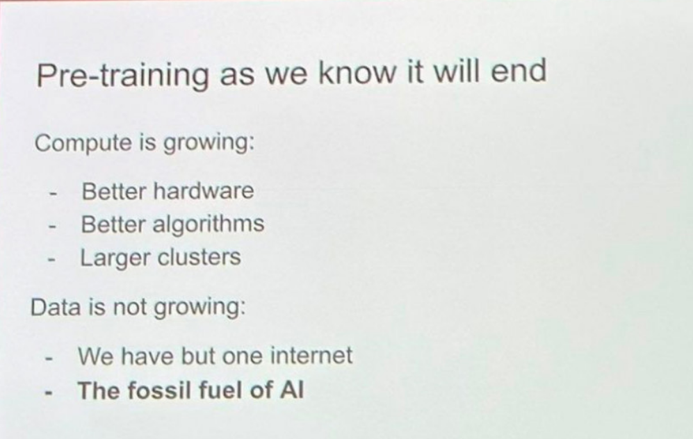
Ilya Sutskever at Neurips 2024
Pre-training as we know it will end.
In industry, most companies focus primarily on prompt engineering, RAG, and fine-tuning, while advanced techniques like pre-training from scratch or deep model customization remain less common due to the significant resources and expertise required.
LLMs, like GPT (Generative Pre-trained Transformer), BERT (Bidirectional Encoder Representations from Transformers), and others, are large-scale models built using the transformer architecture. These models are trained on vast amounts of text data to learn patterns in language, enabling them to generate human-like text, answer questions, summarize information, and perform other natural language processing tasks.
This chapter delves into transformer models, drawing on insights from The Annotated Transformer and Tracing the Transformer in Diagrams, to explore their underlying architecture and practical applications.
7.1. Transformer Architecture
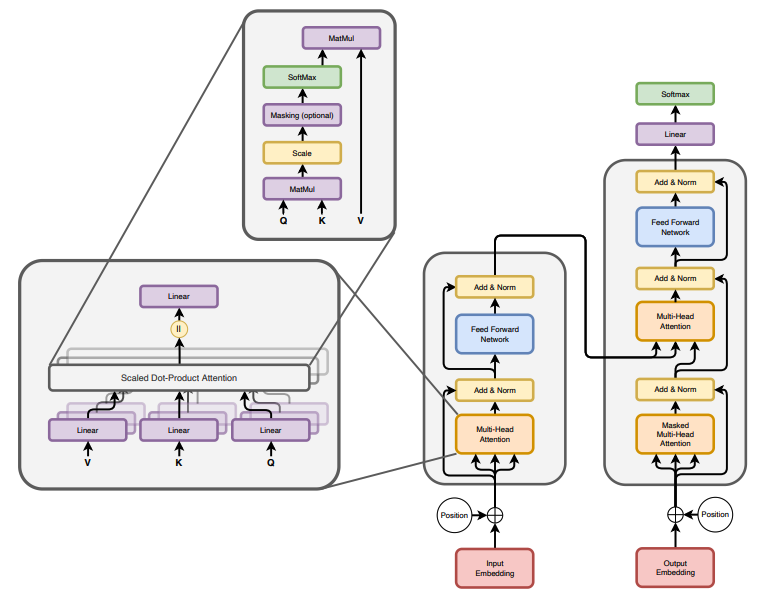
Transformer Architecture (source: [attentionAllYouNeed])
7.1.1. Attention Is All You Need
The Transformer is a deep learning model designed to handle sequential data, such as text, by relying entirely on attention mechanisms rather than recurrence or convolution. It consists of an encoder-decoder structure, where the encoder transforms an input sequence into a set of rich contextual representations, and the decoder generates the output sequence by attending to these representations and previously generated tokens. Both encoder and decoder are composed of stacked layers, each featuring multi-head self-attention (to capture relationships between tokens), feedforward neural networks (for non-linear transformations), and residual connections with layer normalization (to improve training stability). Positional encodings are added to token embeddings to retain sequence order information, and the architecture’s parallelism and scalability make it highly efficient for tasks like machine translation, summarization, and language modeling.
When the Transformer architecture was introduced in the paper “Attention Is All You Need” (Vaswani et al., 2017), the primary task it aimed to address was machine translation. The researchers wanted to develop a model that could translate text from one language to another more efficiently and effectively than the existing sequence-to-sequence (Seq2Seq) models, which relied heavily on recurrent neural networks (RNNs) or long short-term memory (LSTM) networks. RNNs / LSTMs suffer from slow training and inference, short-term memory, and vanishing / exploding gradients challenges, due to their sequentual nature and long-range dependencies. The Transformer with self-attention mechanism achieved to eliminate the sequential bottleneck of RNNs while retaining the ability to capture dependencies across the entire input sequence.
7.1.2. Encoder-Decoder
Transformer has an encoding component, a decoding component, and connections between them. The encoding component is a stack of encoders - usually 6-12 layers, though it can go higher (e.g. T5-large has 24 encoder layers). The decoder component is a stack of decoders, usually in the same number of layers for balance.
Each encoder layer includes multi-head self-attention, feedforward neural network (FNN), add & norm, and positional encoding. It reads the input sequence (e.g., a sentence in Chinese) and produces a context-aware representation.
Each decoder layer includes masked multi-head self-attention, encoder-decoder attention, feedforward neural network (FFN), add & norm, and positional encoding. It generates the output sequence (e.g., a translation in English) using the encoder’s output and previously generated tokens.
The encoder-decoder structure was inspired by earlier Seq2Seq models (Sutskever et al., 2014), which used separate RNNs or LSTMs for encoding the input sequence and decoding the output sequence. The innovation of the Transformer was replacing the recurrent nature of those models with an attention-based approach. The Transformer revolutionized not just machine translation but also the entire field of natural language processing (NLP). Its encoder-decoder structure provided a blueprint for subsequent models:
Encoder-only models (e.g., BERT, RoBERTa, DistilBERT) for understanding tasks such as classification, sentiment analysis, named entity recognition, and question answering.
Unlike encoder-decoder or decoder-only models, encoder-only models don’t generate new sequences. Its architecture and training objectives are optimized for extracting contextual representations from input sequences. They focus solely on understanding and representing the input.
Encoder-only models typically use bidirectional self-attention, meaning each token can attend to all other tokens in the sequence (both before and after it). This contrasts with decoder-only models, which use causal masking and can only attend to past tokens. Bidirectionality provides a more holistic understanding of the input.
Encoder-only models are often pretrained with tasks like masked language modeling (MLM), where random tokens in the input are masked and the model learns to predict them based on context.
Decoder-only models (e.g., GPT series, Transformer-XL) for text generation tasks.
Decoder-only models are trained with an autoregressive objective, meaning they predict the next token in a sequence based on the tokens seen so far. This makes them inherently suited for producing coherent, contextually relevant continuations.
The self-attention mechanism in decoder-only models is causal, meaning each token attends only to previous tokens (including itself). They are pretrained with causal language modeling (CLM), where they learn to predict the next token given the previous ones.
Decoder-only models are not constrained to fixed-length outputs and can generate sequences of arbitrary lengths, making them ideal for open-ended tasks such as story writing, dialogue generation, and summarization.
Encoder-decoder models (e.g., Original Transformer, BART, T5) for sequence-to-sequence tasks such as machine translation, summarization, and text generation.
Encoder and decoder are designed to handle different parts of the task - creating a contextual representation and generating output sequence. This decoupling of encoding and decoding allows the model to flexibly handle inputs and outputs of different lengths.
The encoder-decoder attention mechanism in the decoder allows the model to focus on specific parts of the encoded input sequence while generating the output sequence. This cross-attention mechanism helps maintain the relationship between the input and output sequences.
In many encoder-decoder models (such as those based on Transformers), the encoder processes the input sequence bidirectionally, meaning it can attend to both preceding and succeeding tokens when creating the representations. This ensures a comprehensive understanding of the input sequence before it is passed to the decoder.
During training, the encoder-decoder model is typically provided with a sequence of input-output pairs (e.g., a Chinese sentence and its English translation). This paired structure makes the model highly suited for tasks like translation, where the goal is to map input sequences in one language to corresponding output sequences in another language.
7.1.3. Positional Encoding
Positional encoding is a mechanism used in transformers to provide information about the order of tokens in a sequence. Unlike recurrent neural networks (RNNs), transformers process all tokens in parallel, and therefore lack a built-in way to capture sequential information. Positional encoding solves this by injecting position-dependent information into the input embeddings.
7.1.3.1. Sinusoidal Positional Encodings
Sinusoidal positional encoding adds a vector to the embedding of each token, with the vector values derived using sinusoidal functions. For a token at position \(pos\) in the sequence and a specific dimension \(i\) of the embedding:
where
\(pos\): Position of the token in the sequence.
\(i\): Index of the embedding dimension.
\(d\): Total dimension of the embedding vector.
The positional encodings are added directly to the token embeddings:
Positional Embedding
7.1.3.2. Rotary Positional Embeddings (RoPE)
Rotary positional embedding is a modern variant that introduces positional information through rotation in a complex vector space. It encodes positional information by rotating the query and key vectors in the attention mechanism using a transformation in a complex vector space. RoPE mitigates the limitations of absolute positional encodings by focusing on relative relationships, enabling smooth transitions and better handling of long sequences. This makes it particularly advantageous in large-scale language models like GPT-4, LLaMA, where long-range dependencies and adaptability are crucial.
Given a token vector \(x\) with positional encoding, RoPE applies a rotation:
where \(R(pos)\) is the rotation matrix determined by the token’s position.
Specifically, for a rotation by an angle \(\theta\), the 2D rotation matrix is
For each pair of dimensions \((x_{even}, x_{odd})\), the rotation is performed as
7.1.3.3. Learnable Positional Encodings
Learnable Positional Encodings are a type of positional encoding used in transformer-based models where the positional information is not fixed (like in sinusoidal encoding) but is learned during training. These encodings are treated as trainable parameters and are updated through backpropagation, just like other parameters in the model.
7.1.3.4. Summary
Feature |
Sinusoidal Positional Encoding |
Rotary Positional Embeddings (RoPE) |
Learnable Positional Encodings |
|---|---|---|---|
Type |
Absolute |
Relative |
Absolute |
Learnable |
No |
No |
Yes |
Advantages |
Fixed, no trainable parameters; Generalizes to unseen sequence lengths; Computationally simple. |
Encodes relative positional relationships; Scales efficiently to long sequences; Smooth handling of long-range dependencies. |
Flexible for task-specific adaptation; Optimized during training. |
Disadvantages |
Fixed, cannot adapt to data; Encodes only absolute positions; Less flexible for relative tasks. |
More complex to implement; Relatively new, less widespread for general tasks. |
Limited to a fixed maximum sequence length; No inherent relative positioning; Requires more parameters. |
Usage |
Early models (e.g., original Transformer); S equence-to-sequence tasks like translation. |
Modern LLMs (e.g., GPT-4, LLaMA) with long context lengths; Tasks requiring long-range dependencies. |
Popular in earlier models like GPT-2, BERT; Tasks with shorter sequences. |
Best For |
Simplicity, generalization to unseen data. |
Long-context tasks, relative dependencies, efficient scaling. |
Task-specific optimization, shorter context tasks. |
7.1.4. Embedding Matrix
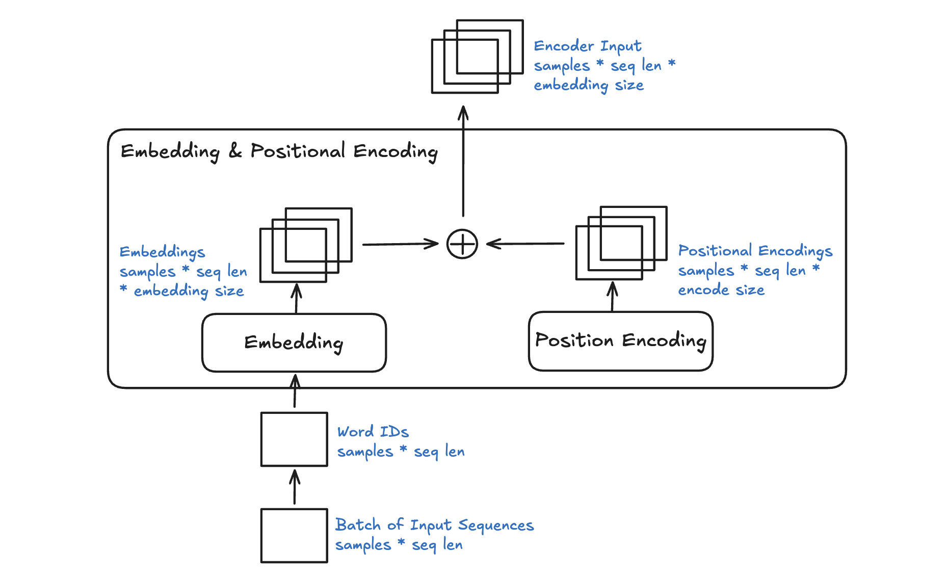
Embedding refers to the process of converting discrete tokens (words, subwords, or characters) into continuous vector representations in a high-dimensional space. These vectors capture the semantic and syntactic properties of tokens, allowing the model to process and understand language more effectively. Embedding layer is a necessary component because:
Discrete symbols are not directly understandable by the model. Embeddings transform these discrete tokens into continuous vectors. Neural networks process continuous numbers more effectively than discrete symbols.
Embeddings help the model learn relationships between words. By learning the semantic properties of tokens during training, words with similar meanings (e.g. “king” and “queen”) should have similar vector representations.
In Transformer based models, embeddings are not just static representations but can be adjusted as the model learns from the context of a sentence to capture subtle semantic nuances and dependencies between words.
Word Embedding
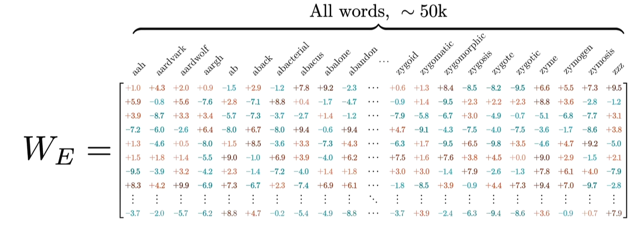
Take an example of embedding matrix \(W_E\) with ~50k vocabulary size, each token in the vocabulary has a corresponding vector, typically initialized randomly at the beginning of training. Embedding matrix does not only represent individual words. They also encode the information about the position of the word. And through training process (passing through self-attention and multiple layers), these embeddings are transformed into contextual embeddings, encoding not only the individual word but also its relationship to other words in the sequence.
The reason why a model predicting the next word requires efficient context incorporation, is that the meaning of a word is clearly informed by its surroundings, sometimes this includes context from a long distance away. For example, with contextual embeddings, the dot products of pieces of this sentence “Harry Potter attends Hogwarts School of Witchcraft and Wizardry, retrieves the Philosopher’s Stone, battles a basilisk, and ultimately leads a final battle at Hogwarts, defeating Voldemort and bringing peace to the wizarding world” results in the following projections in embedding space:
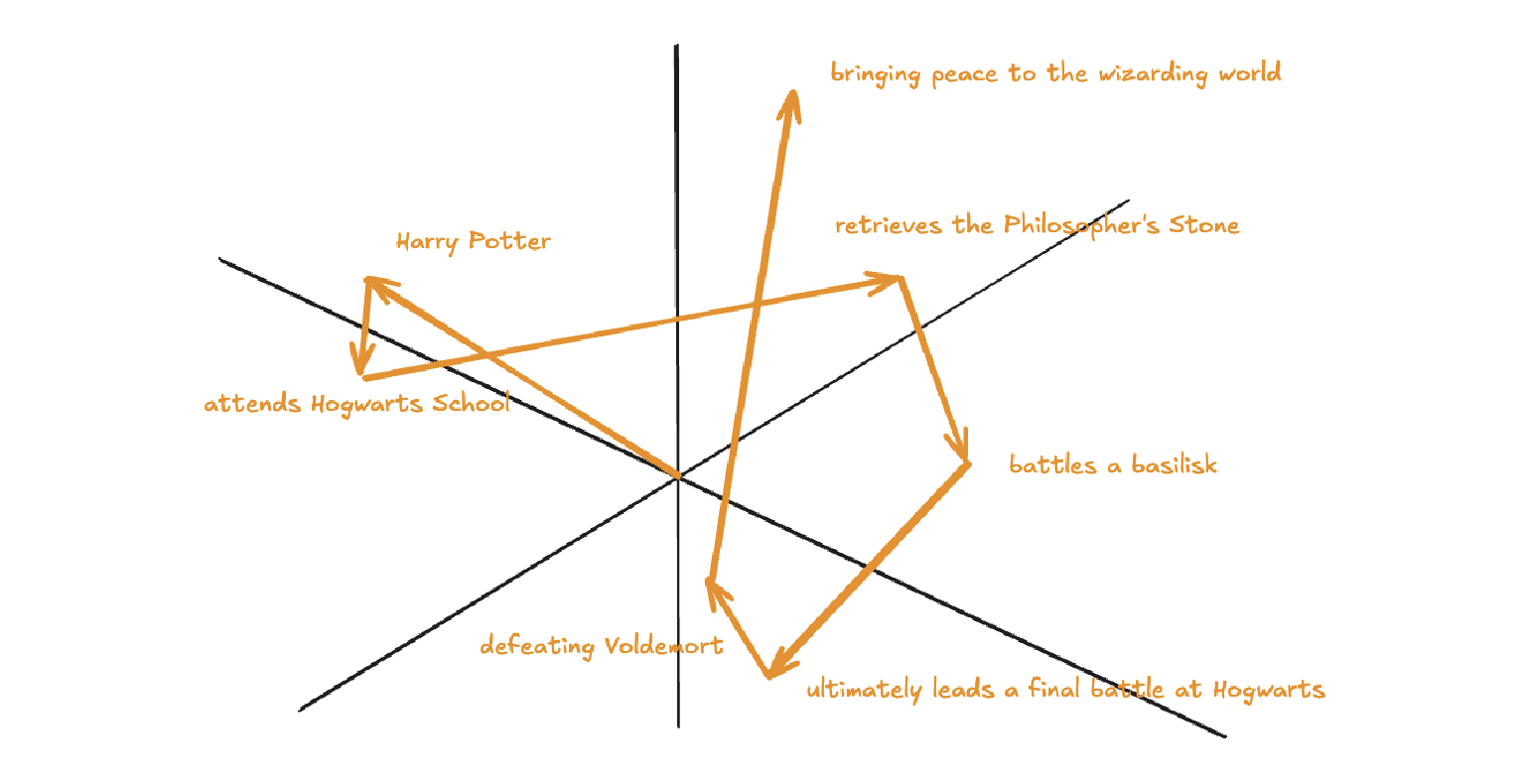
Contextual Embedding
Embedding matrix contains vectors of all words in the vocabulary. It’s the first pile of weights in our model. If the vocabulary size is \(V\) and the embedding dimension is \(d\), the embedding matrix \(W_E\) has dimensions \(d \times V\). The total number of parameters in this embedding matrix is calculated by \(d \times V\).
7.1.5. Attention Mechanism
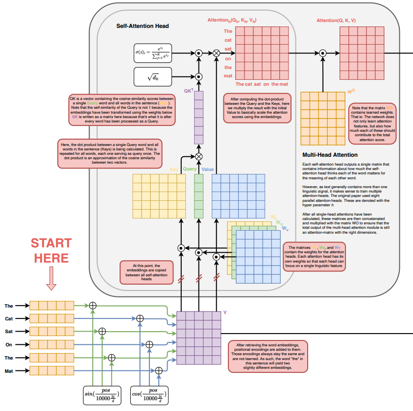
Self Attention (source: The Transformer Architecture A Visual Guide)
7.1.5.1. Self-Attention
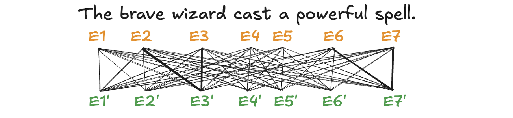
A self-attention is called single-head attention, which enables the model to effectively capture relationships and dependencies between different tokens within the same input sequence. Multi-headed attention has multiple self-attentions running in parallel. The goal of self-attention is to produce a refined embedding where each word has ingested contextual meanings from other words by a series of computations. For example, in the input of “The brave wizard cast a powerful spell”, the refined embedding E3’ of ‘wizard’ should contain the meaning of ‘brave’, and the refined embedding E7’ of ‘spell’ should contain the meaning of ‘powerful’.
The computation involved in self-attention in transformers consists of several key steps: generating query, key, and value representations, calculating attention scores, applying softmax, and computing a weighted sum of the values.
Linear Projection to Query space
Given an input represention with dimension of \((d \times N)\) where \(d\) is the embedding dimension and \(N\) is the token number. Query matrix \(W_Q\) with dimension of \((N \times d_q)\) (\(d_q\) is usually small e.g. 128) contains learnable parameters. It is used to project input representation \(W_E\) to the smaller query space \(Q\) by matrix multiplication.
\[\begin{split}Q &= W_E W_Q\\ (N\times d)(d\times d_q) &\rightarrow (N \times d_q)\end{split}\]Conceptually, the query matrix aims to ask each word a question regarding what kinds of relationship it has with each of the other words.
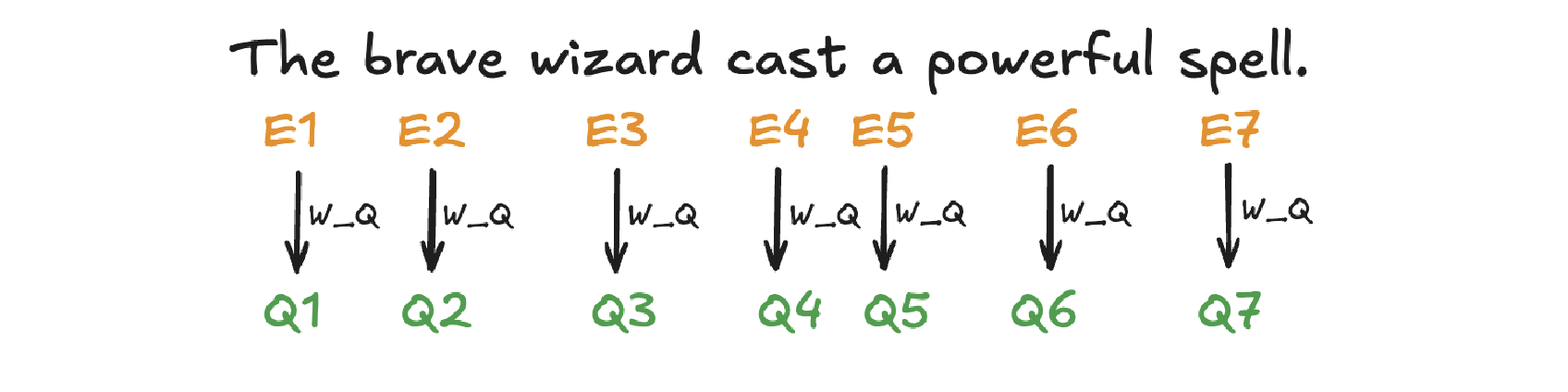
Query Projection
Linear Projection to Key space
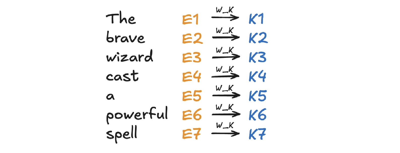
Key matrix \(W_k\) with dimension of \((N \times d_k)\) contains learnable parameters. It is used to project input representation \(W_E\) to the smaller key space \(K\) by matrix multiplication.
\[\begin{split}K &= W_E W_K \\ (N \times d) (d \times d_k) &\rightarrow (N \times d_k)\end{split}\]Conceptually, the keys are answering the queries by matching the queries whenever they closely align with each other. In our example of “The brave wizard cast a powerful spell”, the key metrix maps the word ‘brave’ to vectors that are closely aligned with the query produced by the word ‘wizard’.
Key Projection
Compute Attention Scores
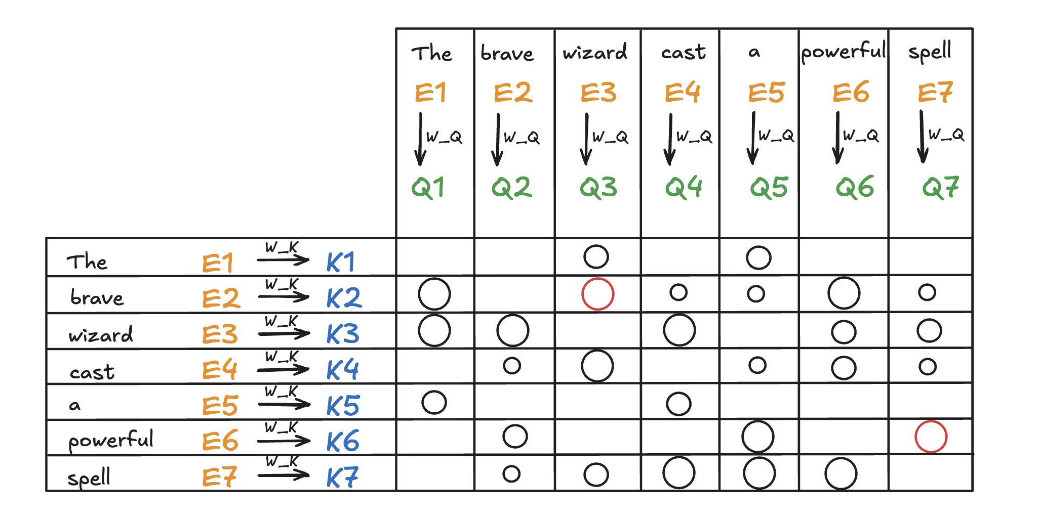
Attention scores are calculated by taking the dot product of the query vectors with the key vectors. These scores as a measurement of relationship represent how well each key matches each query. They can be values from negative infinity to positive infinity.
\[\text{Attention Score} = QK^T\]In our example, the attention score produced by \(K_2 \cdot Q_3\) is expected to be a large positive value because ‘brave’ is an adjective to ‘wizard’. In other words, the embedding of ‘brave’ attends to the embedding of ‘wizard’.
Attention Score
Scaling and softmax normalization
To prevent large values in the attention scores (which could lead to very small gradients), the scores are often scaled by the square root of the dimension of the key vectors \(\sqrt{d_k}\). This scaling helps stabilize the softmax function used in the next step.
\[\text{Scaled Attention Score} = {QK^T \over \sqrt{d_k}}\]The attention scores are passed through a softmax function, which normalizes them into a probability distribution. This ensures that each column of the attention matrix sums to 1, so each token has a clear distribution of “attention” over all tokens.
\[\text{Attention Weights} = \text{softmax}\Big({QK^T\over{\sqrt{d_k}}}\Big)\]Note that for a masked self attention, the bottom left triangle of attention scores are set to negative infinity before softmax normalization. The purpose is to mask those information as latter words are not allowed to influence earlier words. After softmax normalization, those masked attention information becomes zero and the columns stay normalized. This process is called masking.
Computing weighted sum of values
In the attention score matrix with dimension of \(N \times N\), each column is giving weights according to how relevant the word in key space (on the left in the figure) is to the correpsonding word in query space (on the top in the figure). This matrix is also called attention pattern.
The size of attention pattern is the square of the context size, therefore, context size is a huge bottleneck for LLMs. Recent years, some variations of attention mechanism are developed such as Sparse Attention Mechanism, Blockwise Attention, Linformer, Reformer, Longformer, etc, aiming to make context more scalable.
Linear Projection to Value space
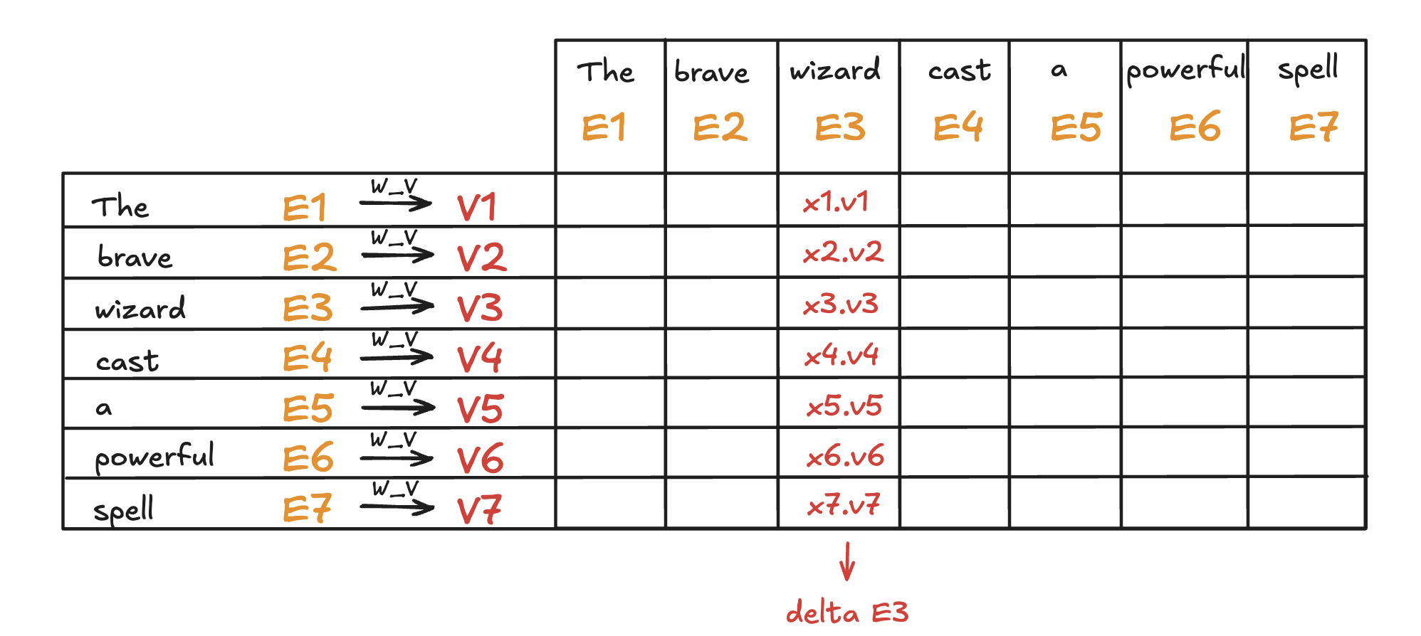
Value matrix \(W_v\) with dimension of \((N \times d_v)\) contains learnable parameters. It is used to project input representation \(W_E\) to the smaller value space \(V\) by matrix multiplication.
\[\begin{split}V &= W_E W_V \\ (N \times d) (d \times d_v) &\rightarrow (N \times d_v)\end{split}\]Conceptually, by maping the embedding of a word to the value space, it’s trying to figure out what should be added to the embedding of other words, if this word is relevant to adjusting the meaning of other words.
Compute Weighted Sum of Values
Each token’s output is computed by taking a weighted sum of the value vectors, where the weights come from the attention distribution obtained in the previous step.
\[\begin{split}\text{Output} &= \text{Attention Weights} \times V\\ (N \times N) (N \times d_v) &\rightarrow (N \times d_v)\end{split}\]This results in a matrix of size \(N \times d_v\) where for each word there is a weighted sum of the value vectors \(\Delta E\) based on the attention distribution. Conceptually, this is the change going to be added to the original embedding, resulting in a more refined vector, encoding contextually rich meaning.
Value Projection and Weighted Sum
To sum up, given \(W_E\) input matrix (\(N \times d\)), \(W_Q, W_K, W_V\) as weight matrices (\(d\times d_q, d\times d_k, d\times d_v\)), the matrix form of the full self-attention process can be written as:
where the final output matrix is \(N \times d_v\).
A full attention block inside a transformer consists of multi-head attention, where self-attention operations run in parallel, each with its own distinct Key, Query, Value matrices.
To update embedding matrix, the weighted sum of values is passed through a linear transformation (via \(W_O\)), and then added to the original input embeddings via a residual connection.
The number of parameters involved in Attention Mechanism:
# Parameters |
|
|---|---|
Embedding Matrix |
d_embed * n_vocab |
Key Matrix |
d_key * d_embed * n_heads * n_layers |
Query Matrix |
d_query * d_embed * n_heads * n_layers |
Value Matrix |
d_value * d_embed * n_heads * n_layers |
Output Matrix |
d_embed * d_value * n_heads * n_layers |
Unembedding Matrix |
n_vocab * d_embed |
7.1.5.2. Cross Attention
Cross-attention is a mechanism in transformers where the queries (\(Q\)) come from one sequence (e.g., the decoder), while the keys (\(K\)) and values (\(V\)) come from another sequence (e.g., the encoder). It allows the model to align and focus on relevant parts of a second sequence when processing the current sequence.
Feature |
Self-Attention |
Cross-Attention |
|---|---|---|
Source of Queries |
Queries (\(Q\)) come from the same sequence. |
Queries (\(Q\)) come from one sequence (e.g., decoder). |
Source of Keys /Values |
Keys (\(K\)) and Values (\(V\)) come from the same sequence. |
Keys (\(K\)) and Values (\(V\)) come from a different sequence (e.g., encoder). |
Purpose |
Captures relationships within the same sequence. |
Aligns and integrates information between two sequences. |
Example Usage |
Used in both encoder and decoder to process input or output tokens. |
Used in encoder-decoder models (e.g., translation) to let the decoder focus on encoder outputs. |
7.1.6. Layer Normalization
Layer Normalization is crucial in transformers because it helps stabilize and accelerate the training of deep neural networks by normalizing the activations across the layers. The transformer architecture, which consists of many layers and complex operations, benefits significantly from this technique for several reasons:
Internal Covariate Shift:
Deep models like transformers often suffer from internal covariate shift, where the distribution of activations changes during training due to the update of model parameters. This can make training slower and less stable.
Layer normalization helps mitigate this by ensuring that the output of each layer has a consistent distribution, which leads to faster convergence and more stable training.
Gradient Flow:
In deep models, the gradients can become either very small (vanishing gradient problem) or very large (exploding gradient problem) as they propagate through the layers. Layer normalization helps keep the gradients within a reasonable range, ensuring efficient gradient flow and preventing these issues.
Improved Convergence:
By normalizing the activations, layer normalization allows the model to use larger learning rates, which speeds up training and leads to better convergence.
Works Across Batch Sizes:
Unlike Batch Normalization, which normalizes activations across the batch dimension, Layer Normalization normalizes across the feature dimension for each individual example, making it more suitable for tasks like sequence modeling, where the batch size may vary and the model deals with sequences of different lengths.
The process can be broken down into the following steps:
Compute the Mean and Variance: for a given input \(x = [x_1, ..., x_d]\):
\[\begin{split}\mu &= {1\over d} \sum^d_{i=1}x_i\\ \sigma^2 &= {1\over d} \sum^d_{i=1} \sum^d_{i=1} (x_i-\mu)^2\end{split}\]where \(\mu\) is the mean and \(\sigma^2\) is the variance of the input.
Normalize the input: subtracting the mean and dividing by the standard deviation:
\[\hat{x_i} = { x_i - \mu \over \sqrt{\sigma^2 + \epsilon}}\]where \(\epsilon\) is a small constant added to the variance to avoid division by zero.
Scale and shift: after normalization, the output is scaled and shifted by learnable parameters \(\gamma\) (scale) and \(\beta\) (shift), which allow the model to restore the original distribution if needed:
\[y_i = \gamma \cdot \hat{x_i} + \beta\]where \(\gamma\) and \(\beta\) are trainable parameters learned during the training process.
7.1.7. Residual Connections
In the transformer architecture, residual connections are used after each key operation, such as:
After Self-Attention: The input to the attention layer is added back to the output of the self-attention mechanism.
After Feed-Forward Networks: Similarly, after the output of the feed-forward network is computed, the input to the feed-forward block is added back to the result.
In both cases, the sum is typically passed through a Layer Normalization operation, which stabilizes the training process further.
Residual connection has the following advantages:
Skip Connection: The original input to the layer is skipped over and added directly to the output of the layer. This allows the model to preserve the information from earlier layers, helping it learn faster and more efficiently.
Enabling Easier Gradient Flow: In deep neural networks, as layers become deeper, gradients can either vanish or explode, making training difficult. Residual connections mitigate the vanishing gradient problem by allowing gradients to flow more easily through the network during backpropagation.
Helping with Identity Mapping: Residual connections allow the network to learn identity mappings. If a certain layer doesn’t need to make any modifications to the input, the network can simply learn to output the input directly, ensuring that deeper layers don’t hurt the performance of the network. This helps the network avoid situations where deeper layers perform worse than shallow layers.
Stabilizing Training: The direct path from the input to the output, via the residual connection, helps stabilize the training by providing an additional gradient flow, making the learning process more robust to initialization and hyperparameters.
7.1.8. Feed-Forward Networks
In the Transformer architecture, Feed-Forward Networks (FFNs) are a key component within each layer of the encoder and decoder. FFNs are applied independently to each token in the sequence, after the attention mechanism (self-attention or cross-attention). They process the information passed through the attention mechanism to refine the representations of each token.
The characteristics and roles of FFN:
Position-Independent: FFNs operate independently on each token’s embedding, without considering the sequence structure. Each token is treated individually.
Non-Linearity: The activation function (like ReLU or GELU) introduces non-linearity into the model, which is crucial for allowing the network to learn complex patterns in the data
Parameter Sharing: The same FFN is applied to each token in the sequence independently. The parameters are shared across all tokens, which is computationally efficient and reduces the number of parameters in the model.
Dimensionality Expansion: The hidden layer size \(d_{ff}\) is typically larger than the model dimension \(d_{\text{model}}\) (often by a factor of 4), allowing the network to learn richer representations in the intermediate space.
Local Information Processing: FFNs only process local information about each token’s embedding, as opposed to the self-attention mechanism, which captures global dependencies across all tokens in the sequence.
Residual Connection: FFNs in transformers use residual connections, where the input to the FFN is added to the output. This helps prevent vanishing gradient issues and makes training deep models more efficient.
Parallelization: Since FFNs are applied independently to each token, they can be parallelized effectively, leading to faster training and inference.
The network can only process a fixed number of vectors at a time, known as its context size. The context size can be 4096 (GPT-3) up to 2M tokens (LongRoPE).
7.1.9. Label Smoothing
In transformer models, label smoothing is commonly applied during the training phase to improve the model’s generalization by modifying the target labels used for training. This technique is typically used in tasks like machine translation, language modeling, and other sequence-to-sequence tasks.
Label smoothing is applied after the decoder generates a probability distribution over the vocabulary in the final layer. The output of the decoder is a vector of logits (raw predictions), which are transformed into a probability distribution using softmax. After applying softmax, the predicted probabilities are compared to the smoothed target distribution to calculate the loss.
The target distribution is originally an one-hot vector. After label smoothing, the one-hot encoding is adjusted so that the correct token has a reduced probability, and the incorrect tokens share a small amount of probability mass. For example, if the origianl one-hot vector is \([0, 1, 0, 0]\), then label smoothing would convert this vector into something like \([0.05, 0.9, 0.05, 0.05]\).
During training, the model computes the cross-entropy loss between the predicted probabilities and the smoothed target distribution. The loss function is modified as follows:
where \(\hat{y_i}\) is the smoothed target probability for class \(i\), and \(p_i\) is the predicted probability for class \(i\).
The model’s output probabilities are then adjusted during training by backpropagating the modified loss. This encourages the model to distribute some probability to alternative tokens, making it less likely to become overly confident in its predictions.
Label smoothing is important in transformers because
Prevents Overfitting: Label smoothing forces the model to spread some probability mass over other tokens, making it less overconfident and more likely to generalize well to unseen data.
Encourages Robustness: By smoothing the target labels, the transformer is encouraged to explore alternative possibilities for each token rather than memorizing the exact sequence of tokens in the training data.
Improved Calibration: The model learns to distribute probability more evenly across all tokens, which often results in better-calibrated probabilities that improve performance in tasks such as classification and sequence generation.
Training Stability: Label smoothing reduces the effect of outliers and noisy labels in the training data, improving the overall stability of training and leading to faster convergence.
7.1.10. Softmax and Temperature
The softmax function is a mathematical operation used to transform a vector of raw scores (logits) into a vector of probabilities. It takes a vector of real numbers, \(z = [z_1, z_2, \dots, z_n]\), and maps it to a probability distribution, where each element is in the range [0, 1], and the sum of all elements equals 1. Mathematically,
The softmax function has been used in GPT in two ways:
Probability Distribution: It converts raw scores into probabilities that sum to 1. Next token as prediction will be the token with the highest probability.
Attention Weights: In attention mechanism, softmax is applied to the score of all tokens in the sequence to normalize them into attention weights.
Properties of Softmax:
Exponentiation: Amplifies the difference between higher and lower scores, making the largest score dominate.
Normalization: Ensures that the output probabilities sum to 1.
Differentiable: Enables backpropagation for training the model.
The temperature parameter is used in the softmax function to control the sharpness or smoothness of the probability distribution over the logits, affecting how confident or diverse the model’s predictions are. When using a temperature \(T > 0\), the logits are scaled by \(\frac{1}{T}\) before applying softmax:
When \(T\) is larger, more weight is given to the lower values, then the distribution is more uniform. If \(T\) is smaller, the biggest logit score will dominate more aggresively. Setting \(T=0\) gives all the weights to the maximum value resulting a ~100% probability. This means higher temperature leads to creative but potentially incoherent outputs, and lower temperature leads to safe and predictable outputs.
7.1.11. Unembedding Matrix
The unembedding matrix in the final layer of GPT is the counterpart to the embedding matrix used at the input layer. GPT’s final hidden layer outputs continuous vectors for each token position in the input sequence. The unembedding matrix projects these vectors into a space where each dimension corresponds to a token in the vocabulary, producing logits for all vocabulary tokens.
The unembedding matrix is not randomly initialized, instead, it’s initialized as the transpose of the embedding matrix \(W_U = W_E^T\). If the vocabulary size is \(V\) and the hidden layer size is \(d\), the unembedding matrix \(W_U\) has dimensions \(V \times d\). In the final layer, GPT produces a hidden state \(h\) with size \(d\) for each token position. The unembedding matrix is applied as follows.
The logits are passed through the softmax function to generate probabilities over the vocabulary. The token with the highest probability (or sampled stochastically) is chosen as the next token.
Using a learned unembedding matrix to compute logits in the final layer of GPT offers critical advantages over directly computing logits from the final hidden vector without this additional projection step:
The embedding and unembedding matrices establish a connection between the input and output token spaces. Without an unembedding matrix, there would be no learned mechanism to align the model’s internal representation to the specific vocabulary used for prediction.
The model’s hidden states are designed to represent rich features of the input sequence rather than being explicitly tied to the vocabulary size. The unembedding matrix translates the compressed hidden state (e.g. 768 or 1024 size) into a vocabulary distribution (e.g. ~50k tokens), ensuring the model can scale to larger vocabularies or output spaces.
The unembedding matrix learns how to transform these rich representations into logits that accurately reflect token probabilities in the specific vocabulary. It provides a structured way for gradients from the loss function (e.g., cross-entropy loss) to update both the model’s hidden representations and the vocabulary mappings.
7.1.12. Decoding
In transformer models, decoding refers to the process of generating output sequences from a model’s learned representations. Decoder takes the hidden state generated by encoder from input representations as well as previously generated tokens (or a start token) and progressively generates the output sequence one by one based on the probability distribution over all possible words in the vocabulary for the next token.
Depending on the specific task and goals (e.g., translation, generation, or summarization), different decoding strategies like beam search, top-k sampling, top-p sampling, and temperature sampling can be used to strike the right balance between creativity and accuracy.
7.1.12.1. Greedy Decoding
Greedy decoding is the simplest and most straightforward method. At each time step, the model chooses the token with the highest probability from the predicted distribution and adds it to the output sequence.
7.1.12.2. Beam Search
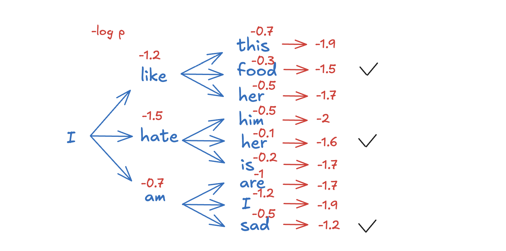
Beam search is a more advanced method than greedy decoding. It keeps track of multiple hypotheses at each decoding step (instead of just the most probable one) and selects the top-k most likely sequences (called the “beam width”).
At each decoding step, beam search explores the top-k candidate sequences (instead of just one) and chooses the one with the highest cumulative probability. A hyperparameter, beam width, controls how many candidate sequences are considered at each step.
Beam Search
7.1.12.3. Top-k Sampling
After the model outputs a probability distribution over the entire vocabulary (e.g., 50,000 tokens for GPT-style models). Only the top \(k\) tokens with the highest probabilities are retained. All other tokens are discarded. The probabilities of the remaining \(k\) tokens are renormalized to sum to 1. A token is randomly selected from the \(k\)-token subset based on the renormalized probabilities.
When \(k=1\), top-k sampling is the same as greedy decoding, where the token with the highest probability is chosen. Higher \(k\) allows more variety by considering more tokens.
Top-k sampling is considered static and predefined because once a contant \(k\) is specified, at each decoding step, only the top \(k\) tokens are considered for sampling. Regardless the shape of distribution, the size of the candidate pool \(k\) does not change. If the probability distribution is “flat”(many tokens with similar probabilities), top-k might still discard important tokens outside the top \(k\). If the distribution is “peaked” (one or a few tokens dominate), top-k might include unlikely tokens unnecessarily.
7.1.12.4. Top-p (Nucleus) Sampling
After the model outputs a probability distribution over the vocabulary. Tokens are sorted in descending order of probability. A cumulative sum of probabilities is calculated for the sorted tokens. The smallest set of tokens whose cumulative probability exceeds or equals \(p\) are retained. The probabilities of the selected tokens are renormalized to sum to 1. A token is randomly selected from this dynamic subset.
When \(p=1\), all tokens are included, then top-p sampling is equivalent to pure sampling. Lower \(p\) focuses on fewer tokens, ensuring higher-quality predictions while retaining some randomness.
Top-p sampling is considered dynamic and adaptive because the number of tokens in the pool varies depending on the shape of the probability distribution. If the distribution is “peaked,” top-p will include fewer tokens because the most probable tokens quickly satisfy the cumulative threshold \(p\). If the distribution is “flat,” top-p will include more tokens to ensure the cumulative probability reaches \(p\).
7.1.12.5. Temperature Scaling
As mentioned in the section “Softmax and Temperature”, temperature scaling is applied to the logits right before sampling or selection (e.g., during top-k or top-p sampling). It modifies the softmax function with a parameter \(T\) added to adjust the shape of the resulting probability distribution from logits. Temperature scaling is used in tasks requiring stochastic decoding methods like top-k sampling or nucleus sampling.
Temperature (:math:`T`) + Top-k:
“High \(T\) + high \(k\)” results in extremely diverse and creative outputs. It may produce incoherent or irrelevant text because too many unlikely tokens are considered. It’s used when generating highly imaginative or exploratory text, such as in creative writing.
“High \(T\) + low \(k\)” balances diversity with some level of coherence. Even with low \(k\), high \(T\) may introduce unexpected word choices. It’s used when creative tasks where some randomness is desired, but the context must still be respected.
“Low \(T\) + high \(k\)” produces coherent and focused outputs because \(T\) emphasizes the most probable tokens. The effect of high \(k\) is mitigated because the scaled probabilities naturally limit diversity.
“Low \(T\) + low \(k\)” produces highly deterministic outputs. Text may seem repetitive. It’s used when tasks requiring consistency, such as factual responses or concise answers.
Temperature (:math:`T`) + Top-p:
“High \(T\) + high \(p\)” produces diverse outputs, but the context may still be loosely followed. It may produce incoherent or irrelevant text because too many unlikely tokens are considered. It’s used when generating exploratory or brainstorming text.
“High \(T\) + low \(p\)” produces constrained output despite high \(T\), as only the most probable tokens within the \(p\)-threshold are considered. Even with low \(k\), high \(T\) may introduce unexpected word choices. It’s used for slightly creative tasks with some emphasis on coherence.
“Low \(T\) + high \(p\)” produces coherent and slightly diverse text. It’s used in balanced tasks, such as assistant chatbots or domain-specific content generation.
“Low \(T\) + low \(p\)” produces very deterministic and rigid outputs. it’s used when generating formal or technical content requiring precision, such as legal or scientific writing.
7.1.12.6. Summary
Method |
Advantages |
Disadvantages |
Use Cases |
|---|---|---|---|
Greedy Decoding |
Simple, fast, deterministic |
May produce repetitive or suboptimal sequences |
When speed is important, low diversity tasks |
Beam Search |
Produces higher-quality sequences, less repetitive |
Computationally expensive, limited by beam width |
Machine translation, summarization |
Top-k Sampling |
Adds diversity, avoids repetitive output |
May reduce coherence in some cases |
Creative text generation, storytelling |
Top-p Sampling |
Dynamically adjusts for diversity, more natural |
May still produce incoherent outputs |
Creative text generation, dialogue systems |
Temperature Sampling |
Fine control over and diversity randomness, balance between coherence |
Requires tuning for optimal results |
Creative text randomness generation, fine-tuning output |
7.2. Modern Transformer Techniques
7.2.1. KV Cache
The primary purpose of the KV cache is to speed up the inference process and make it more efficient. Specifically, during autoregressive generation (such as generating text one token at a time), the transformer model processes the input tokens sequentially, which means that for each new token, it needs to compute the attention scores between the current token and all previous tokens.
Instead of recalculating the key (K) and value (V) vectors for the entire sequence at each step (which would be computationally expensive), the KV cache allows the model to reuse the keys and values from previous tokens, thus reducing redundant computations.
As demonstrated in the diagram below, during the training process, attention scores are calculated by this formula without KV Cache:

When generating the next token during inference, the model doesn’t need to recompute the keys and values for the tokens it has already processed. Instead, it simply retrieves the stored keys and values from the cache for all previously generated tokens. Only the new token’s key and value are computed for the current timestep and added to the cache.
During the attention computation for each new token, the model uses both the new key and value (for the current token) and the cached keys and values (for all previous tokens). This way, the attention mechanism can still compute the correct attention scores and weighted sums without recalculating everything from scratch.
The attention formula with Cache: for a new token \(t\),
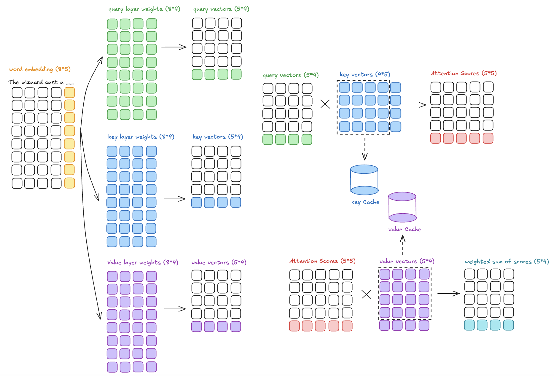
Why Not Cache Queries: Queries are specific to the token being processed at the current step of generation. For every new token in autoregressive decoding, the query vector needs to be freshly computed because it is derived from the embedding of the current token. Keys and values, on the other hand, represent the context of the previous tokens, which remains the same across multiple steps until the sequence is extended.
Space complexity of KV Cache is huge without optimization: The space complexity is calculated by number of layers * number of batch size * number of attention heads * attention head size * sequence length.
Space complexity can be optimized by reducing “number of attention heads” without too much penalty on performance.
7.2.2. Multi-Query Attention
Multi-Query Attention (MQA) is a variant of the attention mechanism introduced to improve the efficiency of transformer models, particularly in scenarios where decoding speed and memory usage are critical. It modifies the standard multi-head attention by using multiple query heads but sharing the key and value matrices across all the heads. There are still multiple independent query heads (\(Q\)), but the key (:math:`K`) and value (:math:`V`) matrices are shared across all the heads.
Each query head \(i\) computes its attention scores with the shared key matrix:
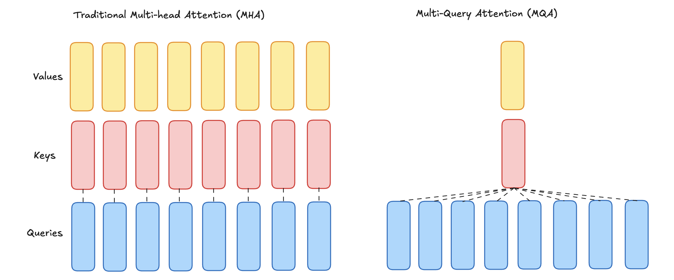
Multi-Query Attention
Advantages of MQA:
Efficiency in Memory Usage: By sharing the \(K\) and \(V\) matrices across heads, the memory footprint is reduced, particularly for the KV cache used during autoregressive generation in large models. This is especially valuable for serving large-scale language models with limited GPU/TPU memory.
Faster Decoding: During autoregressive decoding (e.g., in GPT-like models), each query needs to attend to the cached keys and values. In standard multi-head attention, this involves accessing multiple \(K\) and \(V\) matrices, which can slow down decoding. In MQA, since only one shared \(K\) and \(V\) matrix is used, the decoding process is faster and more streamlined
Minimal Performance Tradeoff: Despite simplifying the model, MQA often achieves comparable performance to standard multi-head attention in many tasks, particularly in large-scale language models.
7.2.3. Grouped-Query Attention
Grouped-Query Attention (GQA) is a hybrid approach between Multi-Head Attention (MHA) and Multi-Query Attention (MQA) that balances computational efficiency and expressivity. In GQA, multiple query heads are grouped together, and each group shares a set of keys and values. This design seeks to retain some of the flexibility of MHA while reducing the memory and computational overhead, similar to MQA.
Mathematically, if there are \(G\) groups, each with \(H / G\) heads, the queries are processed independently for each group but share keys and values within the group:
where \(i\) is the query head within a group.
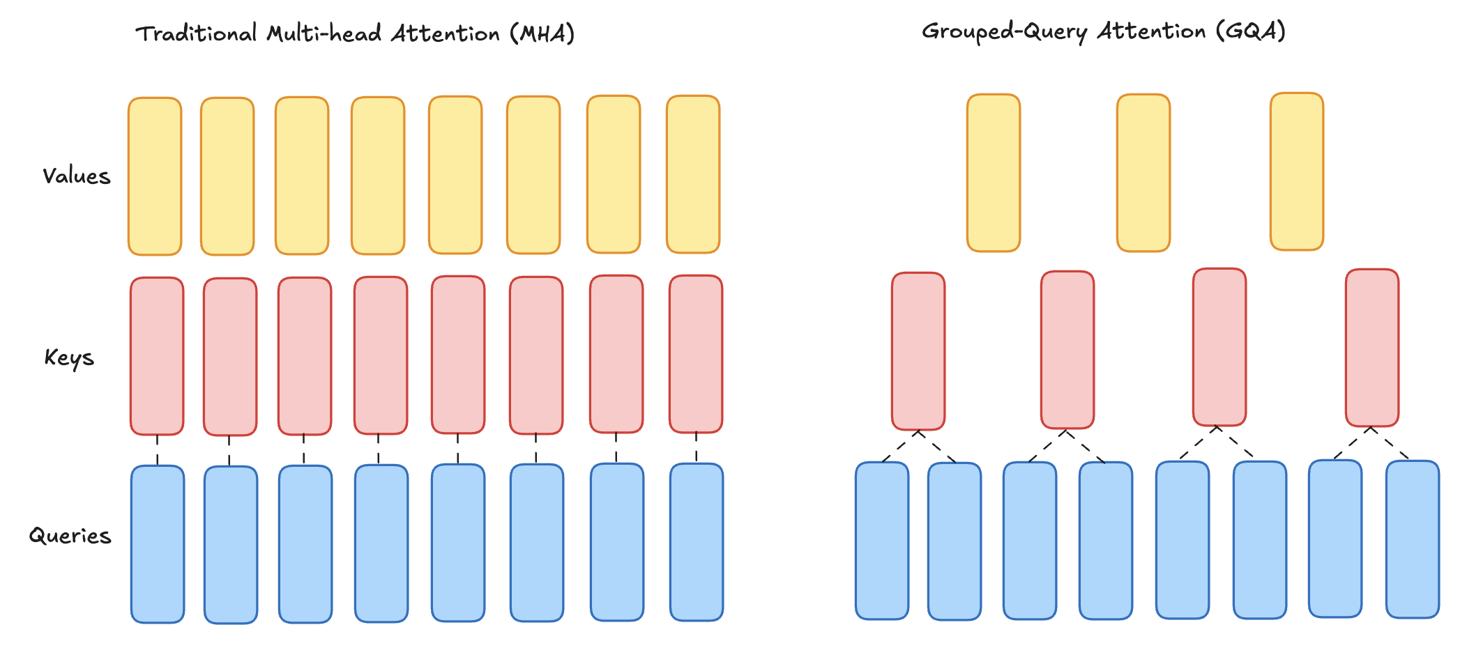
Grouped Query Attention
Advantages of GQA:
Efficiency:
Reduced KV Cache Size: GQA requires fewer key and value matrices compared to MHA. This reduces memory usage, especially during autoregressive decoding when keys and values for all previous tokens are stored in a cache.
Faster Inference: By reducing the number of keys and values to process, GQA speeds up attention computations during decoding, particularly in long-sequence tasks.
Balance Between Flexibility and Efficiency:
More Expressivity Than MQA: Unlike MQA, where all heads share the same keys and values, GQA allows multiple groups of keys and values, enabling more flexibility for the attention mechanism to learn diverse patterns.
Simpler Than MHA: GQA is less computationally expensive and memory-intensive than MHA, as fewer sets of keys and values are used.
Scalability:
GQA is well-suited for very large models and long-sequence tasks where standard MHA becomes computationally and memory prohibitive.
7.2.4. Flash Attention
FlashAttention [Tri_Dao_1] is a novel and efficient algorithm designed to address the computational and memory challenges of self-attention in Transformers, particularly for long sequences. It’s designed to solve two challenges of traditional Transformer implementation:
Self-attention mechanisms in transformers are computationally expensive with quadratic time (\(n^2\)) and memory complexity concerning sequence length (\(n\)), making them inefficient for long sequences.
It’s been revealed in “Data Movement is All You Need” [Andrei] that the key bottleneck during training a Transformer is data movement (reading and writing data) rather than computation. The paper highlights that many transformer operations are memory-bandwidth-bound, meaning that the speed of data transfer to and from HBM often becomes a bottleneck rather than the GPU’s raw computational power. This finding shows that existing implementations of Transformers do not efficiently utilize GPUs.
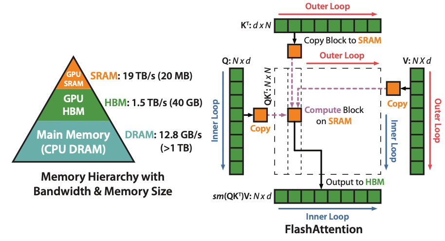
Flash Attention (source: Flash Attention)
The idea of Flash Attention is computing by blocks to reduce HBM reads and writes. Their implementation is a fused CUDA kernel for fine-grained control of memory accesses with two techniques:
Tiling: Tiling works by decomposing large softmax into smaller ones by scaling. It firstly loads inputs by blocks from HBM to SRAM for fast computation, computes attention output with respect to that block in SRAM, then updates output in HBM by scaling.
The method decomposes softmax as follows as an example. \([x_1, x_2]\) represents the concatenation of two partitions (blocks) of input scores. Softmax is independently computed one block at a time. This block-wise operations reduce memory and computational overhead compared to processing the entire sequence at once. \(m(x)\) represents the maximum value within a block of the attention matrix. It’s used as a max-shifting step during the softmax calculation, which improves numerical stability. \(\ell(x)\) is a normalization factor used to convert the exponentials into probability distributions. The combination of scaling factors ensures that the results match the global Softmax computation if it were performed over the full sequence.
\[\begin{split}&m(x) = m(\begin{bmatrix}x_1 & x_2\end{bmatrix}) = \max(m(x_1), m(x_2))\\ &f(x) = \begin{bmatrix} e^{m(x_1)-m(x)}f(x_1) & e^{m(x_2)-m(x)}f(x_2)\end{bmatrix}\\ &\ell(x) = \ell(\begin{bmatrix}x_1 & x_2\end{bmatrix}) = e^{m(x_1)-m(x)}f(x_1)+e^{m(x_2)-m(x)}f(x_2)\\ &\text{softmax}(x) = {f(x)\over \ell(x)}\end{split}\]Recomputation: the idea is to store the output \(\text{softmax}(PQ^T)V\) and softmax normalization factors \(m(x), \ell(x)\) rather than storing the attention matrix from forward in HBM, then recompute the attention matrix in the backward in SRAM.
Recomputation allows the model to discard intermediate activations during the forward pass, only keeping the most essential data for backpropagation. This frees up memory, enabling the model to process much longer sequences or use larger batch sizes. It essentially trades additional computation for reduced memory usage, making the process scalable. This is a tradeoff that is often acceptable, especially with hardware accelerators (GPUs/TPUs) where computation power is abundant but memory capacity is limited.
Both tiling and recomputation aim to address memory and computational challenges when working with large models or long sequences, each improving efficiency in different ways:
Benefit |
Tiling |
Recomputation |
|---|---|---|
Memory Efficiency |
Reduces memory usage by processing smaller tiles instead of the whole sequence at once. |
Saves memory by not storing intermediate results; recomputes when needed. |
Computational Speed |
Enables parallel processing of smaller tiles, improving computation time. |
Reduces memory footprint, potentially increasing throughput by minimizing the need to store large intermediate values. |
Handling Long Sequences |
Makes it feasible to process long sequences that otherwise wouldn’t fit in memory. |
Allows for computation of large models with limited memory by recomputing expensive intermediate steps. |
Hardware Utilization |
Optimizes the use of limited memory resources (e.g., GPU/TPU) by limiting the amount of data in memory. |
Helps avoid running out of memory by not requiring large storage for intermediate states. |
Scalability |
Enables handling of larger datasets and longer sequences without overwhelming memory. |
Makes it possible to work with large models and datasets by not storing every intermediate result. |
Reduced Memory Bandwidth |
Lowers memory bandwidth requirements by only loading small parts of data at a time. |
Minimizes the need for frequent memory writes/reads, improving memory access efficiency. |
Reduces Redundant Computation |
Focuses on smaller sub-problems, reducing redundant operations. |
Recomputes intermediate steps only when necessary, avoiding unnecessary storage and computation. |
Flash Attention 2:
FlashAttention-2 [Tri_Dao_2] builds upon FlashAttention by addressing suboptimal work partitioning between different thread blocks and warps on the GPU. It reduces the number of non-matrix multiplication (matmul) FLOPs, which are slower to perform on GPUs. It also parallelizes the attention computation across the sequence length dimension, in addition to the batch and number of heads dimensions. This increases occupancy (utilization of GPU resources), especially when the sequence is long and the batch size is small. Within each thread block, FlashAttention-2 distributes the work between warps to reduce communication through shared memory. FlashAttention-2 also uses a minor tweak to the backward pass, using the row-wise logsumexp instead of both the row-wise max and row-wise sum of exponentials in the softmax. It incorporates techniques like swapping the order of loops and parallelization over the sequence length, which were first suggested in the Triton implementation. Furthermore, it can also efficiently handle multi-query attention (MQA) and grouped-query attention (GQA) by manipulating indices instead of duplicating key and value heads.
FlashAttention-3:
FlashAttention-3 [Jay_Shah] further improves performance, especially on newer GPUs like the H100. It achieves this by exploiting asynchrony and low-precision computations. It uses a warp-specialized software pipelining scheme that splits the producers and consumers of data into separate warps, overlapping overall computation and data movement. This hides memory and instruction issue latencies. FlashAttention-3 overlaps non-GEMM operations involved in softmax with the asynchronous WGMMA instructions for GEMM. This is done by interleaving block-wise matmul and softmax operations, and by reworking the FlashAttention-2 algorithm to circumvent sequential dependencies between softmax and GEMMs. It implements block quantization and incoherent processing that leverages hardware support for FP8 low-precision to achieve further speedup. FP8 FlashAttention-3 is also more accurate than a baseline FP8 attention by 2.6x, due to its block quantization and incoherent processing, especially in cases with outlier features. It uses primitives from CUTLASS, such as WGMMA and TMA abstractions. Like FlashAttention and FlashAttention-2, it is also able to handle multi-query attention (MQA) and grouped-query attention (GQA).
7.2.5. Mixture of Experts (MoE)
7.2.5.1. Introduction
Mixture of Experts (MoE) is a machine learning architecture designed to enhance model efficiency and scalability by dividing a task among multiple specialized sub-networks, called “experts.” These experts focus on specific subsets of the input data, while a gating network dynamically selects the most relevant expert(s) for each input. This selective activation allows MoE models to significantly reduce computational costs compared to traditional dense neural networks, as only a subset of experts is utilized for any given task.
The concept of MoE originated in the 1991 paper Adaptive Mixture of Local Experts by Robert Jacobs and colleagues. This early work proposed training separate networks (experts) for different regions of the input space, with a gating network determining which expert to activate. The approach demonstrated faster training and improved specialization compared to conventional models.
Modern implementations of MoE have become integral to deep learning, particularly in large-scale models like transformers. Sparse MoE architectures, such as Google’s GShard and Switch Transformers, use conditional computation to activate only a few experts per input, enabling efficient scaling to billions of parameters. These advancements have been pivotal in applications like natural language processing (e.g., Mixtral and DeepSeek), computer vision, and recommendation systems.
7.2.5.2. Methodology
Two main components define a MoE:
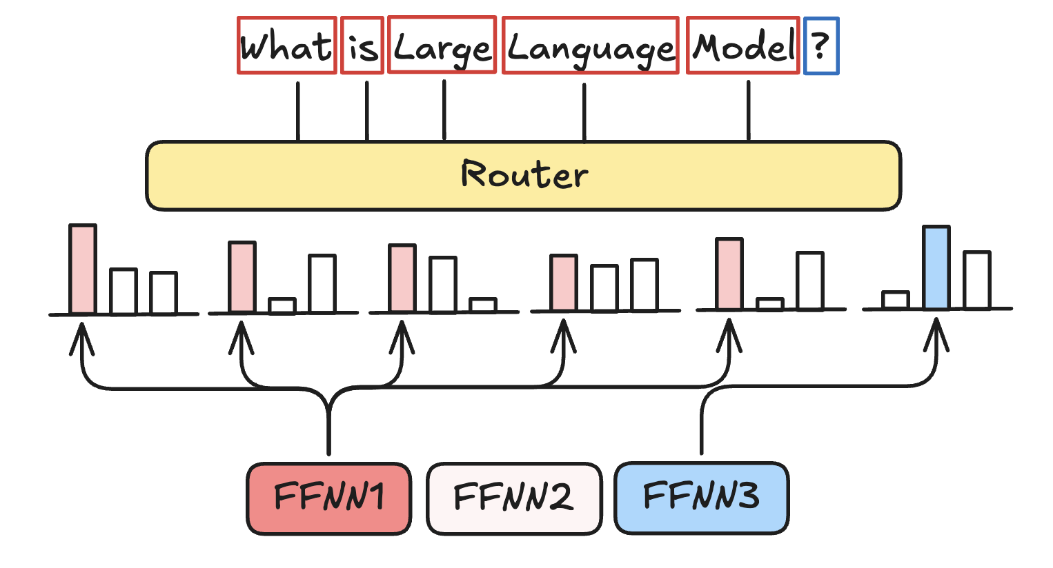
Experts: Experts are Feed Forward Neural Networks (FFNN), and at least one can be activated. Each layer of MoE has a set of experts who learn syntactic information on a token level.
Router (gate network): Router determines which tokens are sent to which experts. It helps to decide which expert is best suited for a given input.
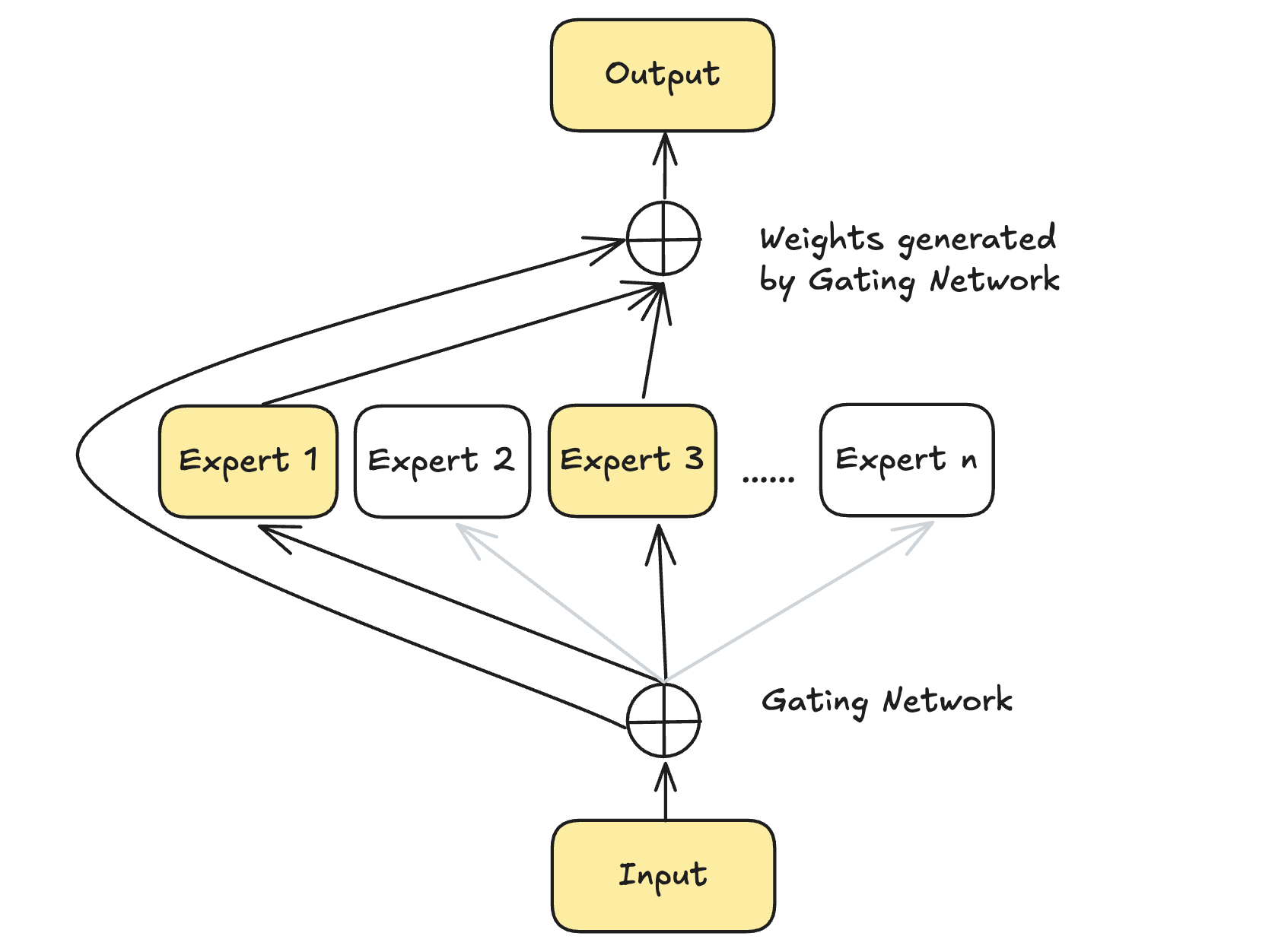
MoE Layer.
In a standard decoder-only transformer architecture, FFNNs are applied after layer normalization. These FFNNs leverage contextual information generated by attention mechanisms to capture complex relationships in the data, with all parameters activated by the input. This layer is also referred to as a dense layer or dense model. MoE replaces these dense layers by segmenting them into multiple smaller components, each acting as an expert, and activates only a subset of experts at any given time. This approach forms a sparse model, where each expert is itself an FFNN.
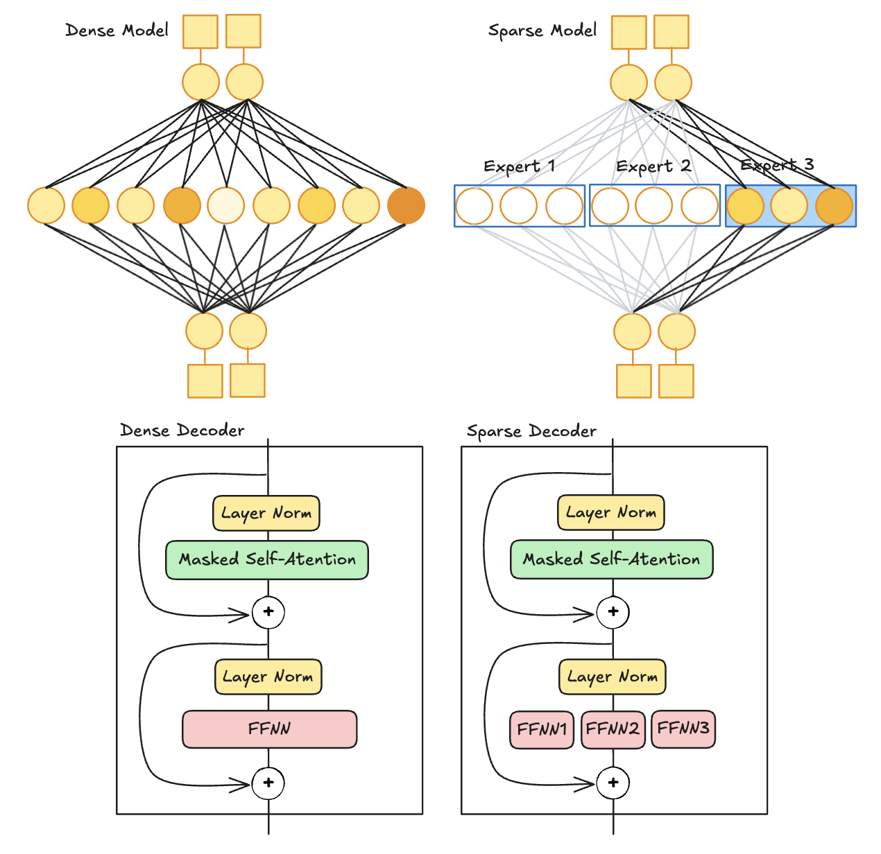
Dense Decoder and Sparse Decoder.
During inference, only specific experts are activated. A given text passes through multiple experts before generating the output. The selected experts may vary for each token, resulting in different paths being taken through the network. Consequently, each token may activate a unique set of experts, ensuring that the most relevant subset is utilized for the input.
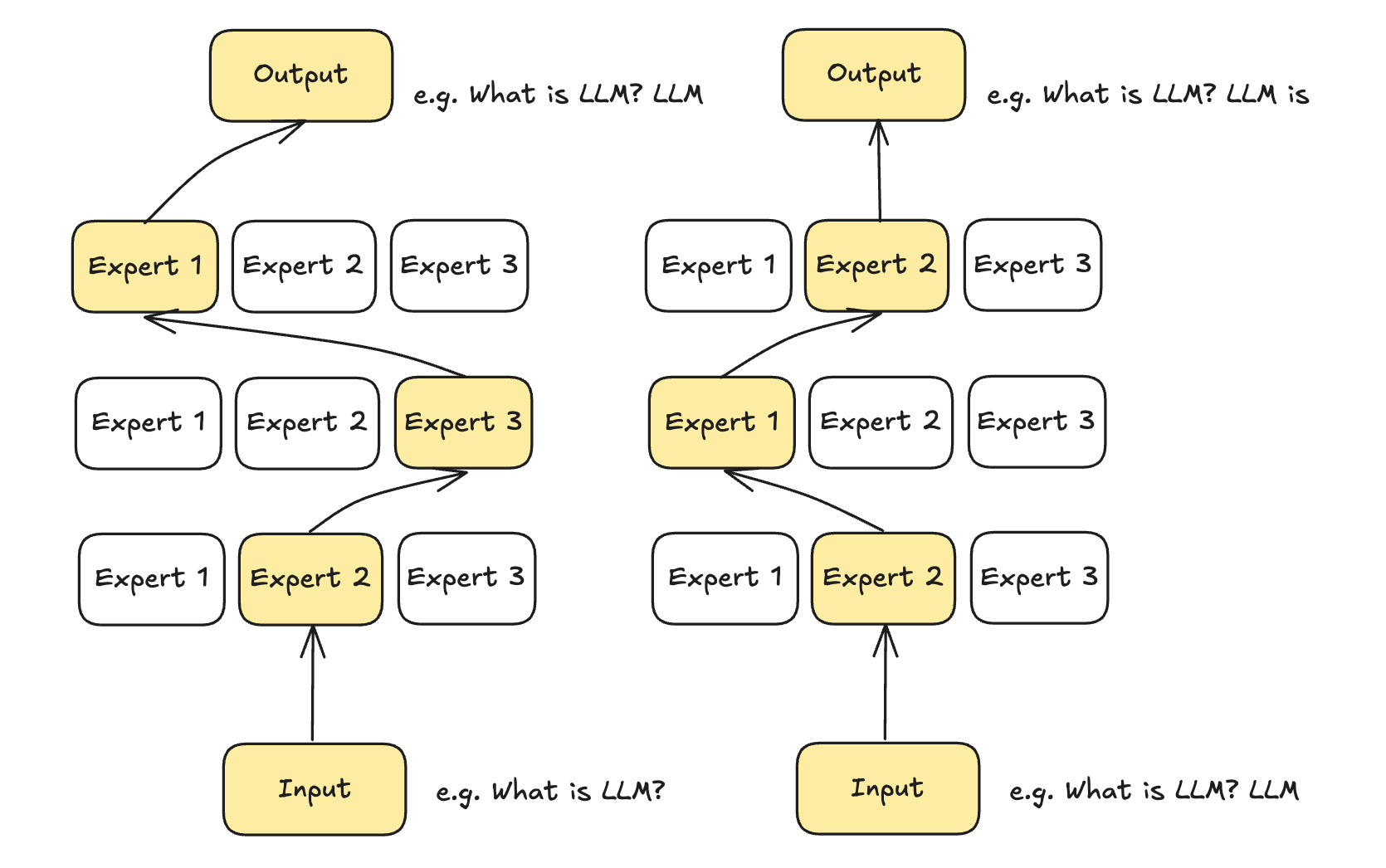
Different tokens have different expert paths.
After passing through the router, a softmax function generates a probability distribution over the experts. This distribution is used to select and activate the most suitable expert(s) for each token. The final output is computed by multiplying the router’s probabilities with the outputs of the selected experts, creating a weighted activation.
Let \(x\) be an input vector. After passing through the router with weights \(W\), we compute \(H(x)\):
The softmax function then computes a probability distribution \(G(x)\) for each expert:
The final output \(y\) is obtained by summing over the selected experts’ outputs weighted by their respective probabilities:
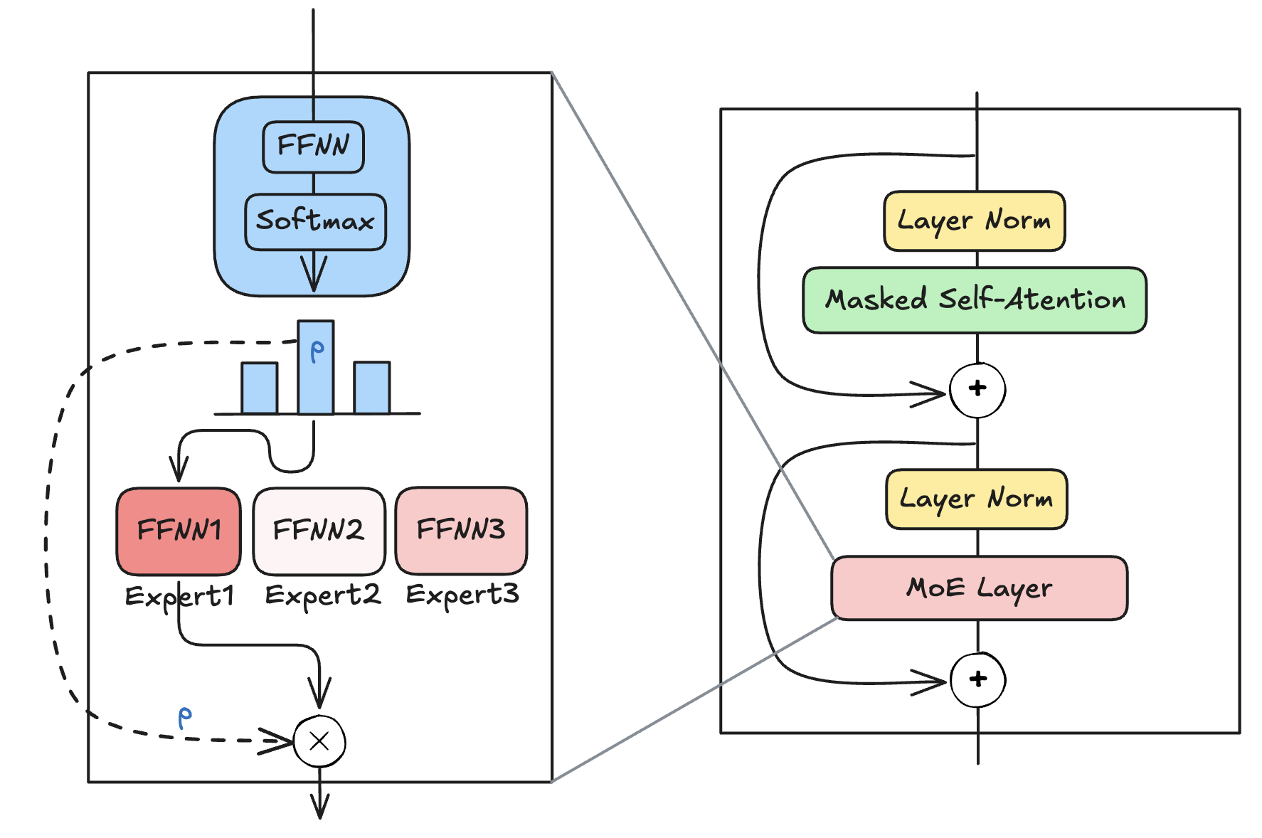
Computations within an MoE layer.
During training, some experts may learn faster than others, leading to an imbalance in their usage regardless of input. This phenomenon, known as load imbalance, can result in overfitting certain experts while underutilizing others. To address this, techniques like KeepTopK introduce trainable Gaussian noise to reduce some experts’ probabilities randomly. Sparsity is enforced by setting all but the top \(K\) expert weights to negative infinity, ensuring that only \(K\) experts are activated per token. Experts with negative infinity router outputs yield zero probabilities after softmax, providing underutilized experts more opportunities to train.
To further enhance load balancing, an auxiliary loss (or load balancing loss) is added alongside the primary network loss. First, importance scores are computed by summing softmax probabilities per expert to measure how often they are chosen. The equality of these scores is quantified using the Coefficient Variation (i.e. standard deviation / mean). Higher CV indicates inequality among expert usage, while lower CV reflects balanced utilization. The auxiliary loss is defined as the product of CV and a scaling factor , and it is minimized during training to promote equal importance among experts and ensure stable training.
Imbalances can also occur in token distribution among experts. For example, one expert may process significantly more tokens than another, leading to undertraining of certain experts. To mitigate this issue, expert capacity limits the number of tokens each expert can process. If an expert reaches its capacity (denoted as \(N\)), additional tokens are routed to other available experts in the layer. If all experts within a layer reach their capacity, subsequent tokens bypass that layer entirely—a phenomenon referred to as token overflow.
Expert Capacity
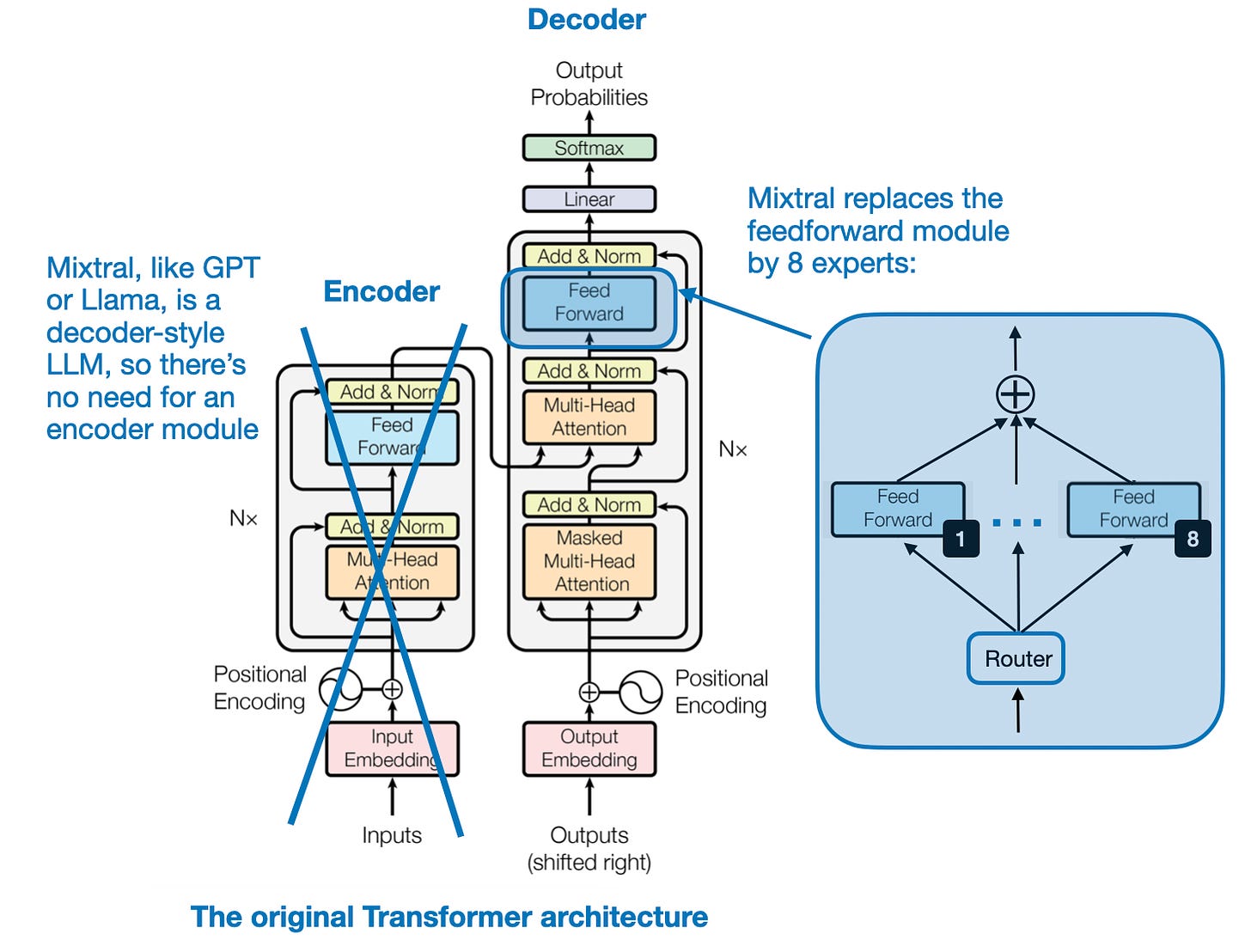
7.2.5.3. Mixtral 8x7B
The Mixtral 8x7B model is a sparse mixture of experts (MoE) model that is currently one of the best performing open-source large language models. The sparse MoE layers allow only a subset of the experts used for each input. Specifically, only 2 experts are used at a time for each input (TopK=2). Mixtral 8x7B replaces each feed-forward module in a transformer architecture with 8 expert layers. It also uses a routing module, or gating network, that directs each token embedding to the 8 expert feed-forward modules. The outputs of these expert layers are then summed.
The “8x” in the name refers to the 8 expert sub-networks and the “7B” indicates that it combines Mistral 7B modules. However, the model’s size is not 56B parameters (8 x 7B). In total, Mixtral 8x7B has 47B parameters. The 7B parameters of the Mistral model are distributed as 1.29B parameters in the attention layers and 5.71B in the feed-forward layers. Mixtral 8x7B has 45.68B parameters in its expert (feed forward) layers. While Mixtral 8x7B has 47B parameters, it only uses 13B parameters for each input token because only two experts are active at a time. This makes it more efficient than a regular, non-MoE 47B parameter model.
Mixtral 8x7B outperforms Llama 2 70B and GPT-3.5 across most benchmarks, including mathematics, code generation, and multilingual tasks, while using significantly fewer active parameters (13B vs. 70B). Its fine-tuned version, Mixtral 8x7B – Instruct, surpasses Claude-2.1, Gemini Pro, and GPT-3.5 Turbo in human evaluation benchmarks, demonstrating superior efficiency, reduced biases, and high performance in long-context and multilingual scenarios.
Mixtral of Experts (Source: Sebastian Raschka)
7.3. Case Studies: DeepSeek-V3
DeepSeek-V3 marks a significant leap forward in AI model performance, offering exceptional inference capabilities that redefine industry benchmarks. The model processes approximately 89 tokens per second, making it nearly 4 times faster than its predecessor, DeepSeek-V2.5, which achieved a rate of 18 tokens per second. This remarkable speed and efficiency position DeepSeek-V3 as a leader in the field.
With an impressive 671 billion Mixture-of-Experts (MoE) parameters, of which 37 billion are activated per token, DeepSeek-V3 operates on a scale unmatched by its predecessor. Its parameter size is approximately 2.8 times larger than DeepSeek-V2.5, and it was trained on a massive dataset of 14.8 trillion high-quality tokens at a total cost of just $5.576 million.
DeepSeek-V3’s exceptional performance stems from a suite of cutting-edge innovations that push the boundaries of AI efficiency and scalability. Key advancements include Multi-Head Latent Attention (MLA), an advanced Mixture-of-Experts (MoE) architecture, and Multi-Token Prediction (MTP), which significantly accelerate text generation by predicting multiple tokens simultaneously. Complementing these are sophisticated training strategies such as the Auxiliary-Loss-Free Load Balancing method, which ensures optimal resource utilization without compromising accuracy, and the FP8 Mixed Precision Framework, designed to reduce memory usage and computational costs while maintaining numerical stability. These technologies collectively enable DeepSeek-V3 to process up to 128,000 tokens in a single context window, a feat that sets new benchmarks for large language models. This unparalleled combination of innovation and efficiency positions DeepSeek-V3 as a formidable competitor in the AI landscape, narrowing the gap between open-source and proprietary systems while redefining standards for scalability and performance. [DeepSeek-V3]
7.3.1. Architecture:
7.3.1.1. Multi-Head Latent Attention (MLA)
Multi-Head Latent Attention (MLA), introduced in DeepSeek-V2, is an innovative attention mechanism designed to address the bottleneck of large Key-Value (KV) caches in traditional Multi-Head Attention (MHA). The core concept of MLA is low-rank joint compression for keys and values, which significantly reduces the KV cache size. During inference, only a compressed latent representation of keys and values is stored, enabling more efficient memory usage and allowing for larger batch sizes and sequence lengths. Additionally, during training, low-rank compression is also applied to queries to minimize activation memory requirements. [DeepSeek-V2]
MLA further incorporates a decoupled Rotary Position Embedding (RoPE), applied to additional multi-head queries and a shared key. This decoupling ensures compatibility with MLA’s compression process by separating positional encoding information from the compressed latent vectors. During inference, the decoupled key is cached alongside the compressed latent vectors, maintaining efficiency while preserving positional context. These innovations make MLA a highly efficient and scalable solution for modern attention mechanisms.
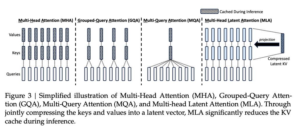
DeepSeek-V2 Multi-Head Latent Attention (MLA) (Source: DeepSeek-V2)
DeepSeekMoE
For Feed-Forward Networks (FFNs), the DeepSeekMoE architecture is utilized, introducing two key innovations to enhance expert specialization and knowledge efficiency. First, Fine-Grained Expert Segmentation divides experts into smaller, more specialized units by splitting the FFN intermediate hidden dimensions. This segmentation enables a more precise decomposition of knowledge while maintaining constant computational costs, allowing for a flexible and adaptive combination of activated experts. Second, Shared Expert Isolation designates specific experts to capture and consolidate common knowledge across contexts. This strategy reduces redundancy among routed experts, ensuring that each expert acquires distinct and focused knowledge for more accurate and efficient processing. DeepSeek-V3 uses the sigmoid function to calculate the affinity scores. It normalizes the selected affinity scores to generate the gating values, ensuring a more balanced and precise distribution.
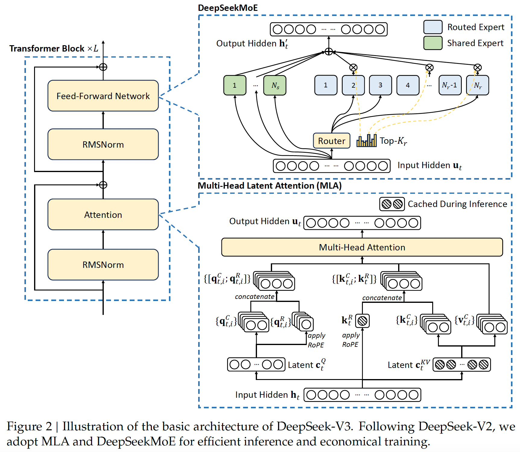
DeepSeekMoE Architecture (Source: DeepSeek-V3)
7.3.1.2. Multi-Token Prediction (MTP)
Multi-Token Prediction (MTP) is an advanced training objective employed in DeepSeek-V3 that extends the model’s ability to predict multiple future tokens simultaneously at each position, rather than focusing on a single token. This approach densifies training signals, improving data efficiency by enabling the model to learn more effectively from the same dataset. Additionally, MTP allows the model to pre-plan its token representations, enhancing its ability to predict long-term patterns and improving performance on complex tasks. Unlike prior implementations, where multiple tokens are predicted in parallel using independent output heads, DeepSeek-V3 sequentially predicts additional tokens while maintaining the full causal chain at each prediction depth. This design preserves contextual dependencies and ensures robust generative capabilities. MTP also accelerates inference by enabling faster token generation and supports speculative decoding for further efficiency gains. These features make MTP a transformative innovation for scaling language models and enhancing their predictive accuracy and speed.
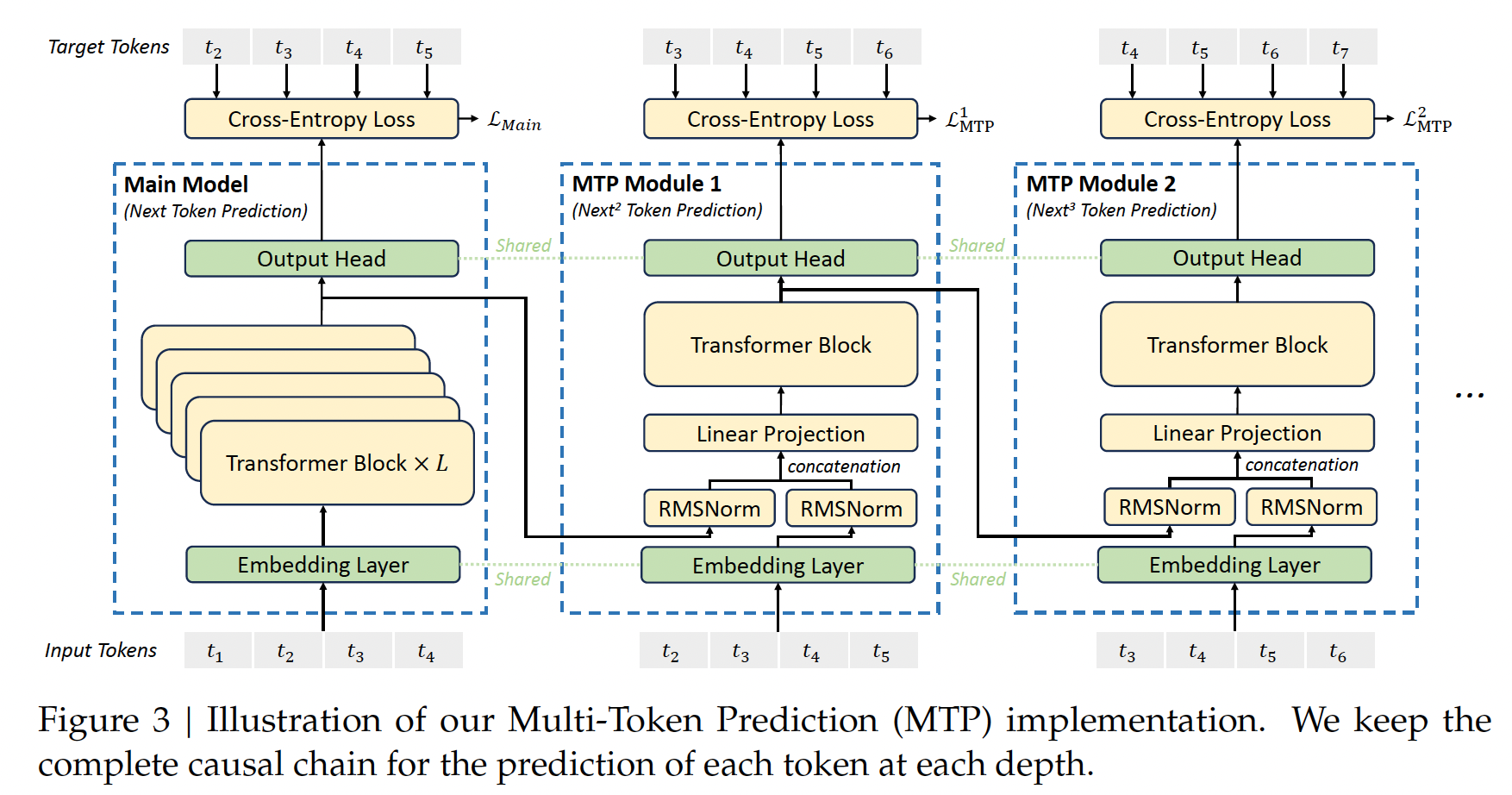
Multi-Token Prediction (MTP) (Source: DeepSeek-V3)
7.3.1.3. Training Strategy:
Auxiliary-Loss-Free Load Balancing
Rather than applying the traditional auxiliary loss for load balancing, they use an auxiliary-lose-free load balancing strategy to achieve a better trade-off between load balance and model performance.
Each expert is assigned a bias term that is added to its affinity score during the routing process. This adjusted score determines the top-K routing decisions. After each training step, the bias for overloaded experts is decreased, while it is increased for underloaded experts. The adjustment rate is controlled by a hyperparameter called the bias update speed \(\gamma\). The bias term is only used for routing decisions, while the gating value (used to scale the FFN output) is derived from the original affinity score, ensuring no interference with model computations.
FP8 Mixed Precision Framework
The mixed precision framework in DeepSeek-V3 leverages FP8 training to significantly enhance computational efficiency and reduce memory usage while maintaining numerical stability. Key features include:
Most compute-intensive operations, such as GEMM (General Matrix Multiplication) operations for forward pass (Fprop), activation backward pass (Dgrad), and weight backward pass (Wgrad), are conducted in FP8 precision. This design doubles computational speed compared to traditional BF16 methods and allows activations to be stored in FP8, reducing memory consumption.
Critical components sensitive to low-precision computations, such as embedding modules, output heads, MoE gating modules, normalization operators, and attention operators, are maintained in higher precision (e.g., BF16 or FP32). This ensures stable training dynamics without compromising efficiency. To further guarantee numerical stability, master weights, weight gradients, and optimizer states are stored in higher precision formats.
To further improve precision in low-precision FP8 training, DeepSeek-V3 incorporates innovative strategies in both quantization and the multiplication process, addressing challenges of accuracy and stability inherent to low-precision formats.
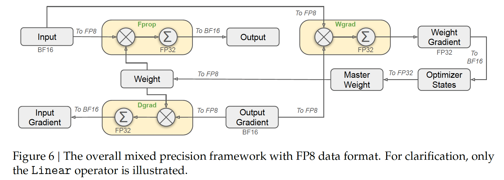
FP Mixed Precision Framework (Source: DeepSeek-V3)