3. Word and Sentence Embedding
Chinese proverb
Though the forms may vary, the essence remains unchanged. – old Chinese proverb
Word embedding is a method in natural language processing (NLP) to represent words as dense vectors of real numbers, capturing semantic relationships between them. Instead of treating words as discrete symbols (like one-hot encoding), word embeddings map words into a continuous vector space where similar words are located closer together.
Colab Notebook for This Chapter
Word Embedding:

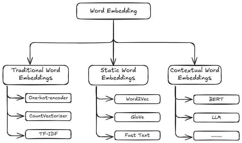
Embedding Diagram
3.1. Traditional word embeddings
Bag of Words (BoW) is a simple and widely used text representation technique in natural language processing (NLP). It represents a text (e.g., a document or a sentence) as a collection of words, ignoring grammar, order, and context but keeping their frequency.
Key Features of Bag of Words:
Vocabulary Creation: - A list of all unique words in the dataset (the “vocabulary”) is created. - Each word becomes a feature.
Representation: - Each document is represented as a vector or a frequency count of words from the vocabulary. - If a word from the vocabulary is present in the document, its count is included in the vector. - Words not present in the document are assigned a count of zero.
Simplicity: - The method is computationally efficient and straightforward. - However, it ignores the sequence and semantic meaning of the words.
Applications:
Text Classification
Sentiment Analysis
Document Similarity
Limitations:
Context Ignorance: - BoW does not capture word order or semantics. - For example, “not good” and “good” might appear similar in BoW.
Dimensionality: - As the vocabulary size increases, the vector representation grows, leading to high-dimensional data.
Sparse Representations: - Many entries in the vectors might be zeros, leading to sparsity.
3.1.1. One Hot Encoder
import numpy as np
import pandas as pd
from collections import Counter
from sklearn.preprocessing import OneHotEncoder

# sample corpus
data = pd.DataFrame({'word':['python', 'pyspark', 'genai', 'pyspark', 'python', 'pyspark']})

# corpus frequency
print('Vocabulary frequency:')
print(dict(Counter(data['word'])))

# corpus order
print('\nVocabulary order:')
print(sorted(set(data['word'])))

# One-hot encode the data
onehot_encoder = OneHotEncoder(sparse_output=False)
onehot_encoded = onehot_encoder.fit_transform(data[['word']])

# the encoded order base on the order of the copus
print('\nEncoded representation:')
print(onehot_encoded)
Vocabulary frequency:
{'python': 2, 'pyspark': 3, 'genai': 1}

Vocabulary order:
['genai', 'pyspark', 'python']

Encoded representation:
[[0. 0. 1.]
[0. 1. 0.]
[1. 0. 0.]
[0. 1. 0.]
[0. 0. 1.]
[0. 1. 0.]]
Note
The detailed PySpark implementation can be found at OneHotEncoder_PySpark.
3.1.2. CountVectorizer
from sklearn.feature_extraction.text import CountVectorizer

# sample corpus
corpus = [
'Gen AI is awesome',
'Gen AI is fun',
'Gen AI is hot'
]

# Initialize the CountVectorizer
vectorizer = CountVectorizer()

# Fit and transform
X = vectorizer.fit_transform(corpus)


print('Vocabulary:')
print(vectorizer.get_feature_names_out())

print('\nEmbedded representation:')
print(X.toarray())
Vocabulary:
['ai' 'awesome' 'fun' 'gen' 'hot' 'is']

Embedded representation:
[[1 1 0 1 0 1]
[1 0 1 1 0 1]
[1 0 0 1 1 1]]
Note
The detailed PySpark implementation can be found at Countvectorizer_PySpark.
To overcome these limitations, advanced techniques like TF-IDF, word embeddings (e.g., Word2Vec, GloVe), and contextual embeddings (e.g., BERT) are often used.
3.1.3. TF-IDF
TF-IDF (Term Frequency-Inverse Document Frequency) is a statistical measure used in text analysis to evaluate the importance of a word in a document relative to a collection (or corpus) of documents. It builds upon the Bag of Words (BoW) model by not only considering the frequency of a word in a document but also taking into account how common or rare the word is across the corpus. The pyspark implementation can be found at [PySpark].
Note
The detailed PySpark implementation can be found at TFIDF_PySpark.
Components of TF-ID
t: the term in corpus.
d: the document.
D: the corpus.
|D|: the length of the corpus or total number of documents.
Document Frequency (DF):
\(DF(t,D)\): the number of documents that contains term \(t\).
- Term Frequency (TF):
Measures how frequently a term appears in a document. The higher the frequency, the more important the term is assumed to be to that document.
Formula:
\[TF(t, d) = \frac{\text{Number of occurrences of term } t \text{ in document } d}{\text{Total number of terms in document } d}\]
- Inverse Document Frequency (IDF):
Measures how important a term is by reducing the weight of common terms (like “the” or “and”) that appear in many documents.
Formula:
\[IDF(t, D) = \log\left(\frac{|D|+1}{DF(t,D) + 1}\right) + 1\]Adding 1 to the denominator avoids division by zero when a term is present in all documents.
Note that the IDF formula above differs from the standard textbook notation that defines the IDF
Note
The IDF formula above differs from the standard textbook notation that defines the IDF as
\[IDF(t) = \log [ |D| / (DF(t,D) + 1) ]).\]
- TF-IDF Score:
The final score is the product of TF and IDF.
Formula:
\[TF\text{-}IDF(t, d, D) = TF(t, d) \cdot IDF(t, D)\]
import pandas as pd
import numpy as np
from collections import Counter
from sklearn.feature_extraction.text import TfidfVectorizer

# sample corpus
corpus = [
'Gen AI is awesome',
'Gen AI is fun',
'Gen AI is hot'
]

# Initialize the TfidfVectorizer
vectorizer = TfidfVectorizer() # norm default norm='l2'

# Fit and transform
X = vectorizer.fit_transform(corpus)

print('Vocabulary:')
print(vectorizer.get_feature_names_out())

# [item for row in matrix for item in row]
corpus_flatted = [item for sub_list in [s.split(' ') for s in corpus]
                     for item in sub_list]

print('\nVocabulary frequency:')
print(dict(Counter(corpus_flatted)))

print('\nEmbedded representation:')
print(X.toarray())
Vocabulary:
['ai' 'awesome' 'fun' 'gen' 'hot' 'is']

Vocabulary frequency:
{'Gen': 3, 'AI': 3, 'is': 3, 'awesome': 1, 'fun': 1, 'hot': 1}

Embedded representation:
[[0.41285857 0.69903033 0.         0.41285857 0.         0.41285857]
[0.41285857 0.         0.69903033 0.41285857 0.         0.41285857]
[0.41285857 0.         0.         0.41285857 0.69903033 0.41285857]]
The above results can be validated by the following steps (IDF in document 1):
# Step 1: Vocabulary  `['ai' 'awesome' 'fun' 'gen' 'hot' 'is']`

tf_idf = pd.DataFrame({'term':vectorizer.get_feature_names_out()})\
         .set_index('term')

# Step 2: |D|
tf_idf['|D|'] = [len(corpus)]*len(vectorizer.get_feature_names_out())

# Step 3: Compute TF for doc 1:  Gen AI is awesome
# - TF for "ai" in Document 1 = 1 (appears once doc 1)
# - TF for "awesome" in Document 1 = 1 (appears once in doc 1)
# - TF for "fun" in Document 1 = 0 (does not appear in doc 1)
# - TF for "gen" in Document 1 = 1 (appear oncein doc 1 )
# - TF for "hot" in Document 1 = 0 (does not appear doc 1 )
# - TF for "is" in Document 1 = 1 (appear once in doc 1 )

tf_idf['TF'] = [1, 1, 0, 1, 0, 1]

# Step 4:  Compute DF for doc 1
# - DF For "ai": Appears in all 3 documents.
# - DF For "awesome": Appears in 1 document.
# - DF For "fun": Appears in 1 document.
# - DF For "Gen": Appears in all 3 documents.
# - DF For "hot": Appears in 1 document.
# - DF For "is": Appears in all 3 documents.

tf_idf['DF'] = [3, 1, 1, 3, 1, 3]

# Step 5: Compute IDF
tf_idf['IDF'] = np.log((tf_idf['|D|']+1)/(tf_idf['DF']+1))+1

# Step 6: Compute TF-IDF
tf_idf['TF-IDF'] = tf_idf['TF']*tf_idf['IDF']

# Step 7: l2 normlization
tf_idf['TF-IDF(l2)'] = tf_idf['TF-IDF']/np.linalg.norm(tf_idf['TF-IDF'])

print(tf_idf)
         |D|  TF  DF       IDF    TF-IDF  TF-IDF(l2)
term
ai         3   1   3  1.000000  1.000000    0.412859
awesome    3   1   1  1.693147  1.693147    0.699030
fun        3   0   1  1.693147  0.000000    0.000000
gen        3   1   3  1.000000  1.000000    0.412859
hot        3   0   1  1.693147  0.000000    0.000000
is         3   1   3  1.000000  1.000000    0.412859
Fun Fact
TfidfVectorizer is equivalent to CountVectorizer followed by TfidfTransformer.
import pandas as pd
import numpy as np
from sklearn.feature_extraction.text import CountVectorizer
from sklearn.feature_extraction.text import TfidfTransformer
from sklearn.pipeline import Pipeline

# sample corpus
corpus = [
'Gen AI is awesome',
'Gen AI is fun',
'Gen AI is hot'
]

# pipeline
pipe = Pipeline([('count', CountVectorizer(lowercase=True)),
               ('tfid', TfidfTransformer())]).fit(corpus)
print(pipe)

# TF
print(pipe['count'].transform(corpus).toarray())

# IDF
print(pipe['tfid'].idf_)
Pipeline(steps=[('count', CountVectorizer()), ('tfid', TfidfTransformer())])
[[1 1 0 1 0 1]
[1 0 1 1 0 1]
[1 0 0 1 1 1]]
[1.         1.69314718 1.69314718 1.         1.69314718 1.        ]
Applications of TF-IDF
Information Retrieval: Ranking documents based on relevance to a query.
Text Classification: Feature extraction for machine learning models.
Document Similarity: Comparing documents by their weighted term vectors.
Advantages
Highlights important terms while reducing the weight of common terms.
Simple to implement and effective for many tasks.
Limitations
Does not capture semantic relationships or word order.
Less effective for very large corpora or when working with very short documents.
Sparse representation due to high-dimensional feature vectors.
For more advanced representations, embeddings like Word2Vec or BERT are often used.
3.2. Static word embeddings
Static word embeddings are word representations that assign a fixed vector to each word, regardless of its context in a sentence or paragraph. These embeddings are pre-trained on large corpora and remain unchanged during usage, making them “static.” These embeddings are usually pre-trained on large text corpora using algorithms like Word2Vec, GloVe, or FastText.
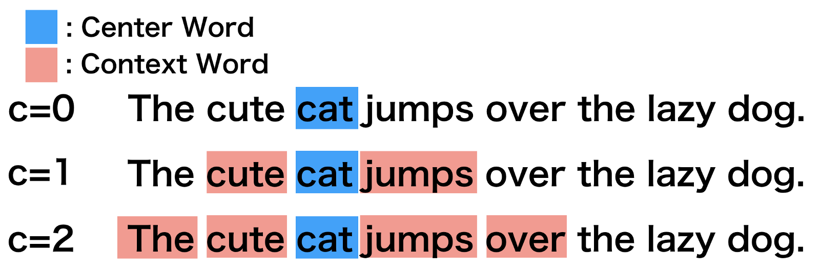
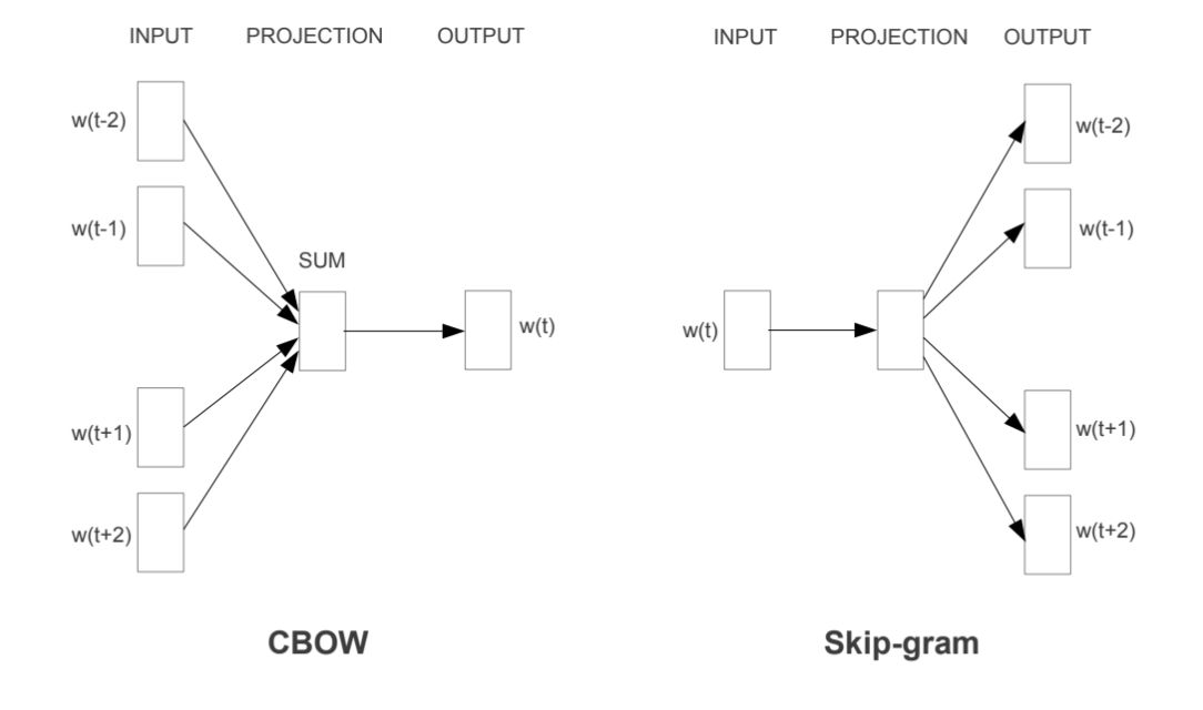
3.2.1. Word2Vec
more details can be found at Chapter 8 Data Manipulation: Features in [PySpark].
Note
The detailed PySpark implementation can be found at Word2Vec_PySpark.
import gensim
from gensim.models import Word2Vec
from nltk.tokenize import sent_tokenize, word_tokenize

# sample corpus
corpus = [
'Gen AI is awesome',
'Gen AI is fun',
'Gen AI is hot'
]


def tokenize_gensim(corpus):

   tokens = []
   # iterate through each sentence in the corpus
   for s in corpus:

      # tokenize the sentence into words
      temp = gensim.utils.tokenize(s, lowercase=True, deacc=False, \
                                    errors='strict', to_lower=False, \
                                    lower=False)

      tokens.append(list(temp))

   return tokens


tokens = tokenize_gensim(corpus)

# Create Word2Vec model
# sg ({0, 1}, optional) – Training algorithm: 1 for skip-gram; otherwise CBOW.
# CBOW
model1 = gensim.models.Word2Vec(tokens, sg=0, min_count=1,
                              vector_size=10, window=5)

# Vocabulary
print(model1.wv.key_to_index)

print(model1.wv.get_normed_vectors())

# Print results
print("Cosine similarity between 'gen' " +
      "and 'ai' - Word2Vec(CBOW) : ",
      model1.wv.similarity('gen', 'ai'))


# Create Word2Vec model
# sg ({0, 1}, optional) – Training algorithm: 1 for skip-gram; otherwise CBOW.
# skip-gram
model2 = gensim.models.Word2Vec(tokens, sg=1, min_count=1,
                              vector_size=10, window=5)

# Vocabulary
print(model2.wv.key_to_index)

print(model2.wv.get_normed_vectors())

# Print results
print("Cosine similarity between 'gen' " +
      "and 'ai' - Word2Vec(skip-gram) : ",
      model2.wv.similarity('gen', 'ai'))
{'is': 0, 'ai': 1, 'gen': 2, 'hot': 3, 'fun': 4, 'awesome': 5}
[[-0.02660277  0.0117296   0.25318226  0.44695902 -0.4615286  -0.35307196
   0.3204311   0.4451589  -0.24882038 -0.18670462]
[ 0.41619968 -0.08647515 -0.2558276   0.3695945  -0.274073   -0.10240843
   0.1622154   0.05593351 -0.46721786 -0.5328355 ]
[ 0.43418837  0.30108306  0.40128633  0.0453006   0.37712952 -0.20221795
-0.05619935  0.34255028 -0.44665098 -0.2337343 ]
[-0.41098067 -0.05088534  0.5218584  -0.40045303 -0.12768732 -0.10601949
   0.44194022 -0.32449666  0.00247097 -0.2600907 ]
[-0.44081825  0.22984274 -0.40207896 -0.20159177 -0.00161115 -0.0135952
-0.3516631   0.44133204  0.2286844   0.423816  ]
[-0.42753762  0.23561442 -0.21681462  0.04321203  0.44539306 -0.23385239
   0.23675178 -0.35568893 -0.18596812  0.49255413]]
Cosine similarity between 'gen' and 'ai' - Word2Vec(CBOW) :  0.32937223
{'is': 0, 'ai': 1, 'gen': 2, 'hot': 3, 'fun': 4, 'awesome': 5}
[[-0.02660277  0.0117296   0.25318226  0.44695902 -0.4615286  -0.35307196
   0.3204311   0.4451589  -0.24882038 -0.18670462]
[ 0.41619968 -0.08647515 -0.2558276   0.3695945  -0.274073   -0.10240843
   0.1622154   0.05593351 -0.46721786 -0.5328355 ]
[ 0.43418837  0.30108306  0.40128633  0.0453006   0.37712952 -0.20221795
-0.05619935  0.34255028 -0.44665098 -0.2337343 ]
[-0.41098067 -0.05088534  0.5218584  -0.40045303 -0.12768732 -0.10601949
   0.44194022 -0.32449666  0.00247097 -0.2600907 ]
[-0.44081825  0.22984274 -0.40207896 -0.20159177 -0.00161115 -0.0135952
-0.3516631   0.44133204  0.2286844   0.423816  ]
[-0.42753762  0.23561442 -0.21681462  0.04321203  0.44539306 -0.23385239
   0.23675178 -0.35568893 -0.18596812  0.49255413]]
Cosine similarity between 'gen' and 'ai' - Word2Vec(skip-gram) :  0.32937223
3.2.2. GloVE
import gensim.downloader as api
# Download pre-trained GloVe model
glove_vectors = api.load("glove-wiki-gigaword-50")
# Get word vectors (embeddings)
word1 = "king"
word2 = "queen"
vector1 = glove_vectors[word1]
vector2 = glove_vectors[word2]
# Compute cosine similarity between the two word vectors
similarity = glove_vectors.similarity(word1, word2)
print(f"Word vectors for '{word1}': {vector1}")
print(f"Word vectors for '{word2}': {vector2}")
print(f"Cosine similarity between '{word1}' and '{word2}': {similarity}")
[==================================================] 100.0% 66.0/66.0MB downloaded
Word vectors for 'king': [ 0.50451   0.68607  -0.59517  -0.022801  0.60046  -0.13498  -0.08813
0.47377  -0.61798  -0.31012  -0.076666  1.493    -0.034189 -0.98173
0.68229   0.81722  -0.51874  -0.31503  -0.55809   0.66421   0.1961
-0.13495  -0.11476  -0.30344   0.41177  -2.223    -1.0756   -1.0783
-0.34354   0.33505   1.9927   -0.04234  -0.64319   0.71125   0.49159
0.16754   0.34344  -0.25663  -0.8523    0.1661    0.40102   1.1685
-1.0137   -0.21585  -0.15155   0.78321  -0.91241  -1.6106   -0.64426
-0.51042 ]
Word vectors for 'queen': [ 0.37854    1.8233    -1.2648    -0.1043     0.35829    0.60029
-0.17538    0.83767   -0.056798  -0.75795    0.22681    0.98587
0.60587   -0.31419    0.28877    0.56013   -0.77456    0.071421
-0.5741     0.21342    0.57674    0.3868    -0.12574    0.28012
0.28135   -1.8053    -1.0421    -0.19255   -0.55375   -0.054526
1.5574     0.39296   -0.2475     0.34251    0.45365    0.16237
0.52464   -0.070272  -0.83744   -1.0326     0.45946    0.25302
-0.17837   -0.73398   -0.20025    0.2347    -0.56095   -2.2839
0.0092753 -0.60284  ]
Cosine similarity between 'king' and 'queen': 0.7839043140411377
3.2.3. Fast Text
Fast Text incorporates subword information (useful for handling rare or unseen words)
from gensim.models import FastText

import gensim
from gensim.models import Word2Vec

# sample corpus
corpus = [
'Gen AI is awesome',
'Gen AI is fun',
'Gen AI is hot'
]


def tokenize_gensim(corpus):

   tokens = []
   # iterate through each sentence in the corpus
   for s in corpus:

      # tokenize the sentence into words
      temp = gensim.utils.tokenize(s, lowercase=True, deacc=False, \
                                    errors='strict', to_lower=False, \
                                    lower=False)

      tokens.append(list(temp))

   return tokens

tokens = tokenize_gensim(corpus)

# create FastText model
model = FastText(tokens, vector_size=10, window=5, min_count=1, workers=4)
# Train the model
model.train(tokens, total_examples=len(tokens), epochs=10)

# Vocabulary
print(model.wv.key_to_index)

print(model.wv.get_normed_vectors())

# Print results
print("Cosine similarity between 'gen' " +
      "and 'ai' - Word2Vec : ",
      model.wv.similarity('gen', 'ai'))
WARNING:gensim.models.word2vec:Effective 'alpha' higher than previous training cycles
{'is': 0, 'ai': 1, 'gen': 2, 'hot': 3, 'fun': 4, 'awesome': 5}
[[-0.01875759  0.086543   -0.25080433  0.2824868  -0.23755953 -0.11316587
   0.473383    0.39204055 -0.30422893 -0.5566626 ]
[ 0.5088161  -0.3323528  -0.128698   -0.11877266 -0.38699347  0.20977001
   0.05947014 -0.05622245 -0.36257952 -0.5177341 ]
[ 0.18038039  0.51484865  0.40694886  0.05965518 -0.05985437 -0.10832689
   0.37992737  0.5992712   0.01503773  0.1192203 ]
[-0.5694013   0.23560704  0.0265804  -0.41392225 -0.00285366 -0.3076269
   0.2076883  -0.425648    0.29903153  0.19965051]
[-0.23892775  0.10744874 -0.03730153 -0.23521401  0.32083488  0.21598674
-0.29570717 -0.03044808  0.75250715  0.26538488]
[-0.31881964 -0.06544963 -0.44274488  0.15485793  0.39120612 -0.05415314
   0.15772066 -0.05987714 -0.6986104   0.03967094]]
Cosine similarity between 'gen' and 'ai' - Word2Vec :  -0.21662527
3.3. Contextual word embeddings
Contextual word embeddings are word representations where the embedding of a word changes depending on its context in a sentence or document. These embeddings capture the meaning of a word as influenced by its surrounding words, addressing the limitations of static embeddings by incorporating contextual nuances.
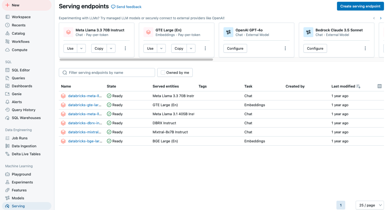
LLMs and Embedding Models in Databricks
3.3.1. BERT
from transformers import BertTokenizer, BertModel
tokenizer = BertTokenizer.from_pretrained('bert-base-uncased')
model = BertModel.from_pretrained("bert-base-uncased")


text = "Gen AI is awesome"
encoded_input = tokenizer(text, return_tensors='pt')
embeddings = model(**encoded_input).last_hidden_state

print(encoded_input)
print({x : tokenizer.encode(x, add_special_tokens=False) for x in ['[CLS]']+ text.split()+ ['[SEP]', '[EOS]']})

print(embeddings.shape)
print(embeddings)
t{'input_ids': tensor([[  101,  8991,  9932,  2003, 12476,   102]]), 'token_type_ids': tensor([[0, 0, 0, 0, 0, 0]]), 'attention_mask': tensor([[1, 1, 1, 1, 1, 1]])}
{'[CLS]': [101], 'Gen': [8991], 'AI': [9932], 'is': [2003], 'awesome': [12476], '[SEP]': [102], '[EOS]': [1031, 1041, 2891, 1033]}


torch.Size([1, 6, 768])
tensor([[[-0.1129, -0.1477, -0.0056,  ..., -0.1335,  0.2605,  0.2113],
         [-0.6841, -1.1196,  0.3349,  ..., -0.5958,  0.1657,  0.6988],
         [-0.5385, -0.2649,  0.2639,  ..., -0.1544,  0.2532, -0.1363],
         [-0.1794, -0.6086,  0.1292,  ..., -0.1620,  0.1721,  0.4356],
         [-0.0187, -0.7320, -0.3420,  ...,  0.4028,  0.1425, -0.2014],
         [ 0.5493, -0.1029, -0.1571,  ...,  0.3503, -0.7601, -0.1398]]],
    grad_fn=<NativeLayerNormBackward0>)
3.3.2. gte-large-en-v1.5
The gte-large-en-v1.5 is a state-of-the-art text embedding model developed
by Alibaba’s Institute for Intelligent Computing. It’s designed for natural
language processing tasks and excels in generating dense vector representations
(embeddings) of text for applications such as text retrieval, classification,
clustering, and reranking.
It can handle up to 8192 tokens, making it suitable for long-context tasks. More details can be found at: https://huggingface.co/Alibaba-NLP/gte-large-en-v1.5 .
# Requires transformers>=4.36.0

import torch.nn.functional as F
from transformers import AutoModel, AutoTokenizer

input_texts = [
'Gen AI is awesome',
'Gen AI is fun',
'Gen AI is hot'
]

model_path = 'Alibaba-NLP/gte-large-en-v1.5'
tokenizer = AutoTokenizer.from_pretrained(model_path)
model = AutoModel.from_pretrained(model_path, trust_remote_code=True)

# Tokenize the input texts
batch_dict = tokenizer(input_texts, max_length=8192, padding=True, \
                     truncation=True, return_tensors='pt')

print(batch_dict)


outputs = model(**batch_dict)
embeddings = outputs.last_hidden_state[:, 0]

# (Optionally) normalize embeddings
embeddings = F.normalize(embeddings, p=2, dim=1)
scores = (embeddings[:1] @ embeddings[1:].T) * 100
print(embeddings)
print(scores.tolist())
{'input_ids': tensor([[  101,  8991,  9932,  2003, 12476,   102],
      [  101,  8991,  9932,  2003,  4569,   102],
      [  101,  8991,  9932,  2003,  2980,   102]]), 'token_type_ids': tensor([[0, 0, 0, 0, 0, 0],
      [0, 0, 0, 0, 0, 0],
      [0, 0, 0, 0, 0, 0]]), 'attention_mask': tensor([[1, 1, 1, 1, 1, 1],
      [1, 1, 1, 1, 1, 1],
      [1, 1, 1, 1, 1, 1]])}

tensor([[ 0.0079,  0.0008, -0.0001,  ...,  0.0418, -0.0138, -0.0236],
      [ 0.0079,  0.0218, -0.0171,  ...,  0.0412, -0.0230, -0.0237],
      [ 0.0073, -0.0106, -0.0194,  ...,  0.0711, -0.0204, -0.0036]],
      grad_fn=<DivBackward0>)
[[92.85284423828125, 92.81655883789062]]
3.3.3. bge-base-en-v1.5
The bge-base-en-v1.5 model is a general-purpose text embedding model developed
by the Beijing Academy of Artificial Intelligence (BAAI). It transforms input text
into 768-dimensional vector embeddings, making it useful for tasks like semantic
search, text similarity, and clustering. This model is fine-tuned using contrastive
learning, which helps improve its ability to distinguish between similar and
dissimilar sentences effectively. More details can be found
at: https://huggingface.co/BAAI/bge-base-en-v1.5 .
from transformers import AutoTokenizer, AutoModel
import torch

# Sentences we want sentence embeddings for
sentences = [
'Gen AI is awesome',
'Gen AI is fun',
'Gen AI is hot'
]
# Load model from HuggingFace Hub
tokenizer = AutoTokenizer.from_pretrained('BAAI/bge-large-zh-v1.5')
model = AutoModel.from_pretrained('BAAI/bge-large-zh-v1.5')
model.eval()

# Tokenize sentences
encoded_input = tokenizer(sentences, padding=True, truncation=True, return_tensors='pt')
print(encoded_input)

# Compute token embeddings
with torch.no_grad():
   model_output = model(**encoded_input)
   # Perform pooling. In this case, cls pooling.
   sentence_embeddings = model_output[0][:, 0]
# normalize embeddings
sentence_embeddings = torch.nn.functional.normalize(sentence_embeddings, p=2, dim=1)
print("Sentence embeddings:", sentence_embeddings)
{'input_ids': tensor([[  101, 10234,  8171,  8578,  8310,   143, 11722,  9974,  8505,   102],
     [  101, 10234,  8171,  8578,  8310,  9575,   102,     0,     0,     0],
     [  101, 10234,  8171,  8578,  8310,  9286,   102,     0,     0,     0]]), 'token_type_ids': tensor([[0, 0, 0, 0, 0, 0, 0, 0, 0, 0],
     [0, 0, 0, 0, 0, 0, 0, 0, 0, 0],
     [0, 0, 0, 0, 0, 0, 0, 0, 0, 0]]), 'attention_mask': tensor([[1, 1, 1, 1, 1, 1, 1, 1, 1, 1],
     [1, 1, 1, 1, 1, 1, 1, 0, 0, 0],
     [1, 1, 1, 1, 1, 1, 1, 0, 0, 0]])}

Sentence embeddings: tensor([[ 0.0700,  0.0119,  0.0049,  ...,  0.0428, -0.0475,  0.0242],
      [ 0.0800, -0.0065, -0.0519,  ...,  0.0057, -0.0770,  0.0119],
      [ 0.0740, -0.0185, -0.0369,  ...,  0.0083, -0.0026,  0.0016]])
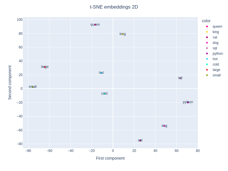
t-SNE embeddings 2D