8. Data Manipulation: Features¶

Chinese proverb

All things are diffcult before they are easy!

Feature building is a super important step for modeling which will determine the success or failure of your model. Otherwise, you will get: garbage in; garbage out! The techniques have been covered in the following chapters, the followings are the brief summary. I recently found that the Spark official website did a really good job for tutorial documentation. The chapter is based on Extracting transforming and selecting features.

8.1. Feature Extraction¶

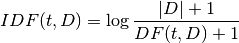
8.1.1. TF-IDF¶

Term frequency-inverse document frequency (TF-IDF) is a feature vectorization method widely used in text mining to reflect the importance of a term to a document in the corpus. More details can be found at: https://spark.apache.org/docs/latest/ml-features#feature-extractors

Stackoverflow TF: Both HashingTF and CountVectorizer can be used to generate the term frequency vectors. A few important differences:

partially reversible (CountVectorizer) vs irreversible (HashingTF) - since hashing is not reversible you cannot restore original input from a hash vector. From the other hand count vector with model (index) can be used to restore unordered input. As a consequence models created using hashed input can be much harder to interpret and monitor.
memory and computational overhead - HashingTF requires only a single data scan and no additional memory beyond original input and vector. CountVectorizer requires additional scan over the data to build a model and additional memory to store vocabulary (index). In case of unigram language model it is usually not a problem but in case of higher n-grams it can be prohibitively expensive or not feasible.
hashing depends on a size of the vector , hashing function and a document. Counting depends on a size of the vector, training corpus and a document.
a source of the information loss - in case of HashingTF it is dimensionality reduction with possible collisions. CountVectorizer discards infrequent tokens. How it affects downstream models depends on a particular use case and data.

HashingTF and CountVectorizer are the two popular alogoritms which used to generate term frequency vectors. They basically convert documents into a numerical representation which can be fed directly or with further processing into other algorithms like LDA, MinHash for Jaccard Distance, Cosine Distance.

$t$ : term
$d$ : document
$D$ : corpus
$|D|$ : the number of the elements in corpus
$TF(t,d)$ : Term Frequency: the number of times that term $t$ appears in document $d$
$DF(t,D)$ : Document Frequency: the number of documents that contains term $t$
$IDF(t, D)$ : Inverse Document Frequency is a numerical measure of how much information a term provides

$IDF(t, D) = \log \frac{|D| + 1}{DF(t, D) + 1}$

$TFIDF(t, d, D)$ the product of TF and IDF

$TFIDF(t, d, D) = TF(t, d) \cdot IDF(t, D)$

Let’s look at the example:

from pyspark.ml import Pipeline
from pyspark.ml.feature import HashingTF, IDF, Tokenizer

sentenceData = spark.createDataFrame([
    (0, "Python python Spark Spark"),
    (1, "Python SQL")],
 ["document", "sentence"])

sentenceData.show(truncate=False)
+--------+-------------------------+
|document|sentence                 |
+--------+-------------------------+
|0       |Python python Spark Spark|
|1       |Python SQL               |
+--------+-------------------------+

Then:

$TF(python,document 1) = 1, TF(spark,document 1) = 2$
$DF(Spark,D)= 2, DF(sql,D)= 1$
IDF:

$IDF(python, D)= \log \frac{|D| + 1}{DF(t, D) + 1} =\log(\frac{2+1}{2+1}) =0$

$IDF(spark, D)= \log \frac{|D| + 1}{DF(t, D) + 1} =\log(\frac{2+1}{1+1}) = 0.4054651081081644$

$IDF(sql, D)= \log \frac{|D| + 1}{DF(t, D) + 1} =\log(\frac{2+1}{1+1}) = 0.4054651081081644$

TFIDF

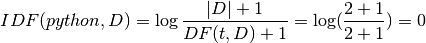
$TFIDF(python, document 1, D) = 3*0 = 0$

$TFIDF(spark, document 1, D) = 2*0.4054651081081644 = 0.8109302162163288$

$TFIDF(sql, document 1, D) = 1*0.4054651081081644 = 0.4054651081081644$

8.1.1.1. Countvectorizer¶

Stackoverflow TF: CountVectorizer and CountVectorizerModel aim to help convert a collection of text documents to vectors of token counts. When an a-priori dictionary is not available, CountVectorizer can be used as an Estimator to extract the vocabulary, and generates a CountVectorizerModel. The model produces sparse representations for the documents over the vocabulary, which can then be passed to other algorithms like LDA.

from pyspark.ml import Pipeline
from pyspark.ml.feature import CountVectorizer
from pyspark.ml.feature import HashingTF, IDF, Tokenizer

sentenceData = spark.createDataFrame([
    (0, "Python python Spark Spark"),
    (1, "Python SQL")],
 ["document", "sentence"])

tokenizer = Tokenizer(inputCol="sentence", outputCol="words")
vectorizer  = CountVectorizer(inputCol="words", outputCol="rawFeatures")

idf = IDF(inputCol="rawFeatures", outputCol="features")

pipeline = Pipeline(stages=[tokenizer, vectorizer, idf])

model = pipeline.fit(sentenceData)

import numpy as np

total_counts = model.transform(sentenceData)\
                    .select('rawFeatures').rdd\
                    .map(lambda row: row['rawFeatures'].toArray())\
                    .reduce(lambda x,y: [x[i]+y[i] for i in range(len(y))])

vocabList = model.stages[1].vocabulary
d = {'vocabList':vocabList,'counts':total_counts}

spark.createDataFrame(np.array(list(d.values())).T.tolist(),list(d.keys())).show()

counts = model.transform(sentenceData).select('rawFeatures').collect()
counts

[Row(rawFeatures=SparseVector(8, {0: 1.0, 1: 1.0, 2: 1.0})),
 Row(rawFeatures=SparseVector(8, {0: 1.0, 1: 1.0, 4: 1.0})),
 Row(rawFeatures=SparseVector(8, {0: 1.0, 3: 1.0, 5: 1.0, 6: 1.0, 7: 1.0}))]

+---------+------+
|vocabList|counts|
+---------+------+
|   python|   3.0|
|    spark|   2.0|
|      sql|   1.0|
+---------+------+

model.transform(sentenceData).show(truncate=False)

+--------+-------------------------+------------------------------+-------------------+----------------------------------+
|document|sentence                 |words                         |rawFeatures        |features                          |
+--------+-------------------------+------------------------------+-------------------+----------------------------------+
|0       |Python python Spark Spark|[python, python, spark, spark]|(3,[0,1],[2.0,2.0])|(3,[0,1],[0.0,0.8109302162163288])|
|1       |Python SQL               |[python, sql]                 |(3,[0,2],[1.0,1.0])|(3,[0,2],[0.0,0.4054651081081644])|
+--------+-------------------------+------------------------------+-------------------+----------------------------------+

from pyspark.sql.types import ArrayType, StringType

def termsIdx2Term(vocabulary):
    def termsIdx2Term(termIndices):
        return [vocabulary[int(index)] for index in termIndices]
    return udf(termsIdx2Term, ArrayType(StringType()))

vectorizerModel = model.stages[1]
vocabList = vectorizerModel.vocabulary
vocabList

['python', 'spark', 'sql']

rawFeatures = model.transform(sentenceData).select('rawFeatures')
rawFeatures.show()

+-------------------+
|        rawFeatures|
+-------------------+
|(3,[0,1],[2.0,2.0])|
|(3,[0,2],[1.0,1.0])|
+-------------------+

from pyspark.sql.functions import udf
import pyspark.sql.functions as F
from pyspark.sql.types import  StringType, DoubleType, IntegerType

indices_udf = udf(lambda vector: vector.indices.tolist(), ArrayType(IntegerType()))
values_udf = udf(lambda vector: vector.toArray().tolist(), ArrayType(DoubleType()))


rawFeatures.withColumn('indices', indices_udf(F.col('rawFeatures')))\
           .withColumn('values', values_udf(F.col('rawFeatures')))\
           .withColumn("Terms", termsIdx2Term(vocabList)("indices")).show()

+-------------------+-------+---------------+---------------+
|        rawFeatures|indices|         values|          Terms|
+-------------------+-------+---------------+---------------+
|(3,[0,1],[2.0,2.0])| [0, 1]|[2.0, 2.0, 0.0]|[python, spark]|
|(3,[0,2],[1.0,1.0])| [0, 2]|[1.0, 0.0, 1.0]|  [python, sql]|
+-------------------+-------+---------------+---------------+

8.1.1.2. HashingTF¶

Stackoverflow TF: HashingTF is a Transformer which takes sets of terms and converts those sets into fixed-length feature vectors. In text processing, a “set of terms” might be a bag of words. HashingTF utilizes the hashing trick. A raw feature is mapped into an index (term) by applying a hash function. The hash function used here is MurmurHash 3. Then term frequencies are calculated based on the mapped indices. This approach avoids the need to compute a global term-to-index map, which can be expensive for a large corpus, but it suffers from potential hash collisions, where different raw features may become the same term after hashing.

from pyspark.ml import Pipeline
from pyspark.ml.feature import HashingTF, IDF, Tokenizer

sentenceData = spark.createDataFrame([
    (0, "Python python Spark Spark"),
    (1, "Python SQL")],
 ["document", "sentence"])

tokenizer = Tokenizer(inputCol="sentence", outputCol="words")
vectorizer  = HashingTF(inputCol="words", outputCol="rawFeatures", numFeatures=5)

idf = IDF(inputCol="rawFeatures", outputCol="features")

pipeline = Pipeline(stages=[tokenizer, vectorizer, idf])


model = pipeline.fit(sentenceData)
model.transform(sentenceData).show(truncate=False)

+--------+-------------------------+------------------------------+-------------------+----------------------------------+
|document|sentence                 |words                         |rawFeatures        |features                          |
+--------+-------------------------+------------------------------+-------------------+----------------------------------+
|0       |Python python Spark Spark|[python, python, spark, spark]|(5,[0,4],[2.0,2.0])|(5,[0,4],[0.8109302162163288,0.0])|
|1       |Python SQL               |[python, sql]                 |(5,[1,4],[1.0,1.0])|(5,[1,4],[0.4054651081081644,0.0])|
+--------+-------------------------+------------------------------+-------------------+----------------------------------+

8.1.2. Word2Vec¶

8.1.2.1. Word Embeddings¶

Word2Vec is one of the popupar method to implement the Word Embeddings. Word embeddings (The best tutorial I have read. The following word and images content are from Chris Bail, PhD Duke University. So the copyright belongs to Chris Bail, PhD Duke University.) gained fame in the world of automated text analysis when it was demonstrated that they could be used to identify analogies. Figure 1 illustrates the output of a word embedding model where individual words are plotted in three dimensional space generated by the model. By examining the adjacency of words in this space, word embedding models can complete analogies such as “Man is to woman as king is to queen.” If you’d like to explore what the output of a large word embedding model looks like in more detail, check out this fantastic visualization of most words in the English language that was produced using a word embedding model called GloVE.

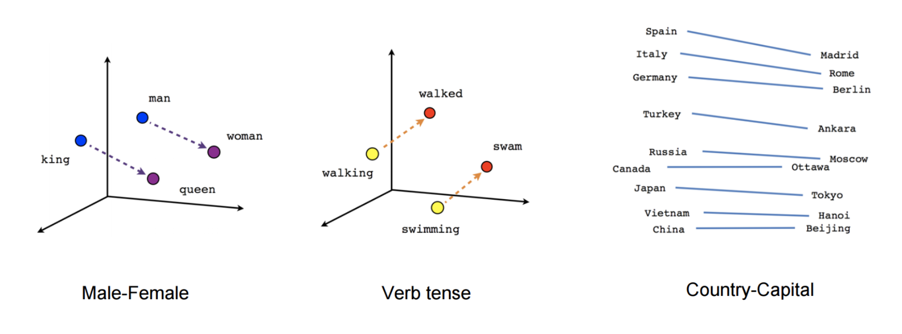
output of a word embedding model¶

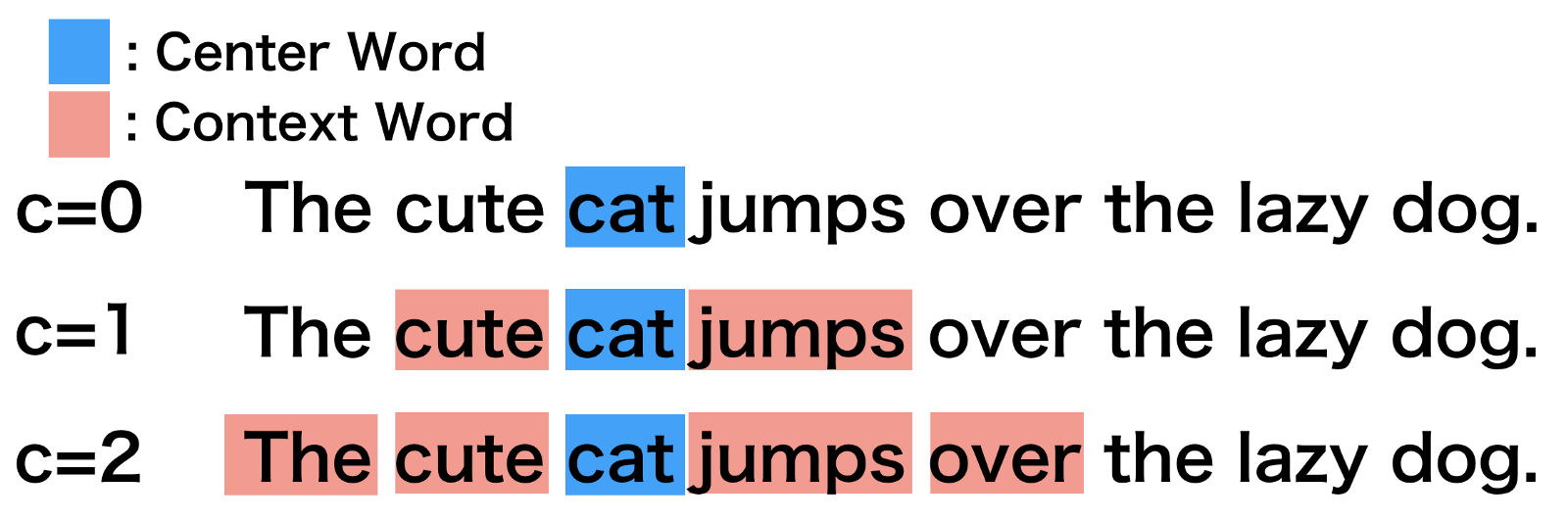
8.1.2.2. The Context Window¶

Word embeddings are created by identifying the words that occur within something called a “Context Window.” The Figure below illustrates context windows of varied length for a single sentence. The context window is defined by a string of words before and after a focal or “center” word that will be used to train a word embedding model. Each center word and context words can be represented as a vector of numbers that describe the presence or absence of unique words within a dataset, which is perhaps why word embedding models are often described as “word vector” models, or “word2vec” models.

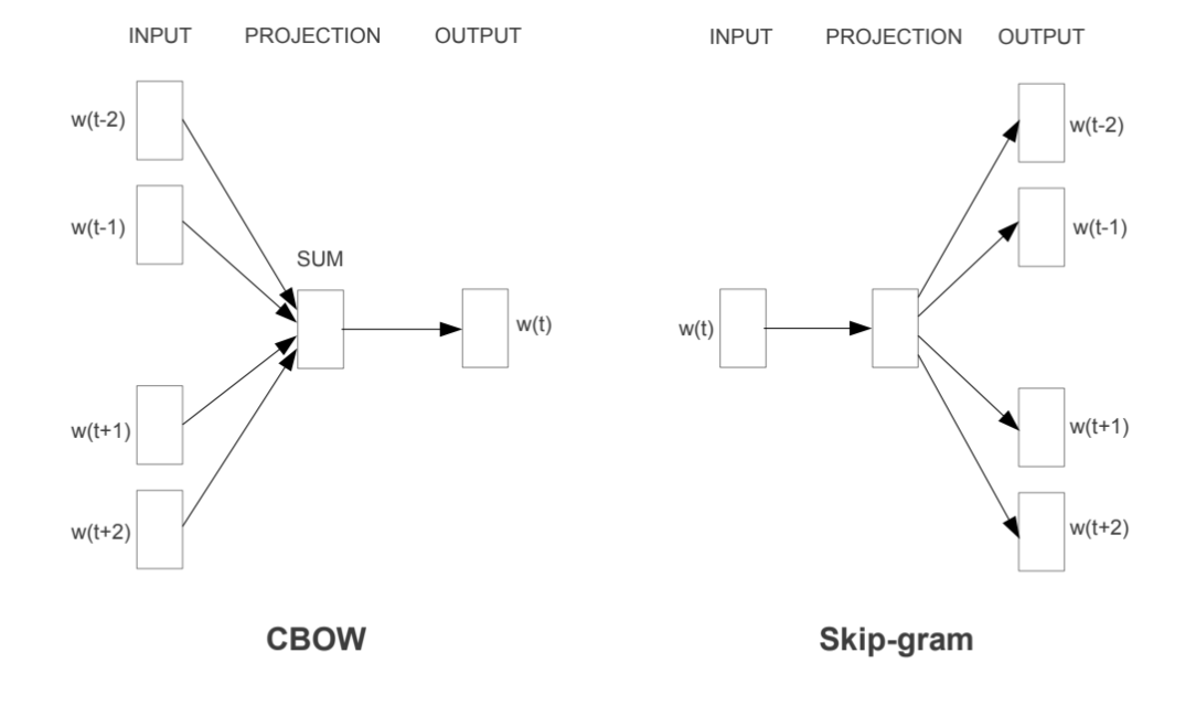
8.1.2.3. Two Types of Embedding Models¶

Word embeddings are usually performed in one of two ways: “Continuous Bag of Words” (CBOW) or a “Skip-Gram Model.” The figure below illustrates the differences between the two models. The CBOW model reads in the context window words and tries to predict the most likely center word. The Skip-Gram Model predicts the context words given the center word. The examples above were created using the Skip-Gram model, which is perhaps most useful for people who want to identify patterns within texts to represent them in multimensional space, whereas the CBOW model is more useful in practical applications such as predictive web search.

8.1.2.4. Word Embedding Models in PySpark¶

from pyspark.ml.feature import Word2Vec

from pyspark.ml import Pipeline

tokenizer = Tokenizer(inputCol="sentence", outputCol="words")
word2Vec = Word2Vec(vectorSize=3, minCount=0, inputCol="words", outputCol="feature")

pipeline = Pipeline(stages=[tokenizer, word2Vec])

model = pipeline.fit(sentenceData)
result = model.transform(sentenceData)

result.show()
+-----+--------------------+--------------------+--------------------+
|label|            sentence|               words|             feature|
+-----+--------------------+--------------------+--------------------+
|  0.0|        I love Spark|    [i, love, spark]|[0.05594437588782...|
|  0.0|       I love python|   [i, love, python]|[-0.0350368790871...|
|  1.0|I think ML is awe...|[i, think, ml, is...|[0.01242086507845...|
+-----+--------------------+--------------------+--------------------+

w2v = model.stages[1]
w2v.getVectors().show()

+-------+-----------------------------------------------------------------+
|word   |vector                                                           |
+-------+-----------------------------------------------------------------+
|is     |[0.13657838106155396,0.060924094170331955,-0.03379475697875023]  |
|awesome|[0.037024181336164474,-0.023855900391936302,0.0760037824511528]  |
|i      |[-0.0014482572441920638,0.049365971237421036,0.12016955763101578]|
|ml     |[-0.14006119966506958,0.01626444421708584,0.042281970381736755]  |
|spark  |[0.1589149385690689,-0.10970081388950348,-0.10547549277544022]   |
|think  |[0.030011219903826714,-0.08994936943054199,0.16471518576145172]  |
|love   |[0.01036644633859396,-0.017782460898160934,0.08870164304971695]  |
|python |[-0.11402882635593414,0.045119188725948334,-0.029877422377467155]|
+-------+-----------------------------------------------------------------+

from pyspark.sql.functions import format_number as fmt
w2v.findSynonyms("could", 2).select("word", fmt("similarity", 5).alias("similarity")).show()

+-------+----------+
|   word|similarity|
+-------+----------+
|classes|   0.90232|
|      i|   0.75424|
+-------+----------+

8.1.3. FeatureHasher¶

from pyspark.ml.feature import FeatureHasher

dataset = spark.createDataFrame([
    (2.2, True, "1", "foo"),
    (3.3, False, "2", "bar"),
    (4.4, False, "3", "baz"),
    (5.5, False, "4", "foo")
], ["real", "bool", "stringNum", "string"])

hasher = FeatureHasher(inputCols=["real", "bool", "stringNum", "string"],
                       outputCol="features")

featurized = hasher.transform(dataset)
featurized.show(truncate=False)

+----+-----+---------+------+--------------------------------------------------------+
|real|bool |stringNum|string|features                                                |
+----+-----+---------+------+--------------------------------------------------------+
|2.2 |true |1        |foo   |(262144,[174475,247670,257907,262126],[2.2,1.0,1.0,1.0])|
|3.3 |false|2        |bar   |(262144,[70644,89673,173866,174475],[1.0,1.0,1.0,3.3])  |
|4.4 |false|3        |baz   |(262144,[22406,70644,174475,187923],[1.0,1.0,4.4,1.0])  |
|5.5 |false|4        |foo   |(262144,[70644,101499,174475,257907],[1.0,1.0,5.5,1.0]) |
+----+-----+---------+------+--------------------------------------------------------+

8.1.4. RFormula¶

from pyspark.ml.feature import RFormula

dataset = spark.createDataFrame(
    [(7, "US", 18, 1.0),
     (8, "CA", 12, 0.0),
     (9, "CA", 15, 0.0)],
    ["id", "country", "hour", "clicked"])

formula = RFormula(
    formula="clicked ~ country + hour",
    featuresCol="features",
    labelCol="label")

output = formula.fit(dataset).transform(dataset)
output.select("features", "label").show()

+----------+-----+
|  features|label|
+----------+-----+
|[0.0,18.0]|  1.0|
|[1.0,12.0]|  0.0|
|[1.0,15.0]|  0.0|
+----------+-----+

8.2. Feature Transform¶

8.2.1. Tokenizer¶

from pyspark.ml.feature import Tokenizer, RegexTokenizer
from pyspark.sql.functions import col, udf
from pyspark.sql.types import IntegerType

sentenceDataFrame = spark.createDataFrame([
    (0, "Hi I heard about Spark"),
    (1, "I wish Java could use case classes"),
    (2, "Logistic,regression,models,are,neat")
], ["id", "sentence"])

tokenizer = Tokenizer(inputCol="sentence", outputCol="words")

regexTokenizer = RegexTokenizer(inputCol="sentence", outputCol="words", pattern="\\W")
# alternatively, pattern="\\w+", gaps(False)

countTokens = udf(lambda words: len(words), IntegerType())

tokenized = tokenizer.transform(sentenceDataFrame)
tokenized.select("sentence", "words")\
    .withColumn("tokens", countTokens(col("words"))).show(truncate=False)

regexTokenized = regexTokenizer.transform(sentenceDataFrame)
regexTokenized.select("sentence", "words") \
    .withColumn("tokens", countTokens(col("words"))).show(truncate=False)

+-----------------------------------+------------------------------------------+------+
|sentence                           |words                                     |tokens|
+-----------------------------------+------------------------------------------+------+
|Hi I heard about Spark             |[hi, i, heard, about, spark]              |5     |
|I wish Java could use case classes |[i, wish, java, could, use, case, classes]|7     |
|Logistic,regression,models,are,neat|[logistic,regression,models,are,neat]     |1     |
+-----------------------------------+------------------------------------------+------+

+-----------------------------------+------------------------------------------+------+
|sentence                           |words                                     |tokens|
+-----------------------------------+------------------------------------------+------+
|Hi I heard about Spark             |[hi, i, heard, about, spark]              |5     |
|I wish Java could use case classes |[i, wish, java, could, use, case, classes]|7     |
|Logistic,regression,models,are,neat|[logistic, regression, models, are, neat] |5     |
+-----------------------------------+------------------------------------------+------+

8.2.2. StopWordsRemover¶

from pyspark.ml.feature import StopWordsRemover

sentenceData = spark.createDataFrame([
    (0, ["I", "saw", "the", "red", "balloon"]),
    (1, ["Mary", "had", "a", "little", "lamb"])
], ["id", "raw"])

remover = StopWordsRemover(inputCol="raw", outputCol="removeded")
remover.transform(sentenceData).show(truncate=False)

+---+----------------------------+--------------------+
|id |raw                         |removeded           |
+---+----------------------------+--------------------+
|0  |[I, saw, the, red, balloon] |[saw, red, balloon] |
|1  |[Mary, had, a, little, lamb]|[Mary, little, lamb]|
+---+----------------------------+--------------------+

8.2.3. NGram¶

from pyspark.ml import Pipeline
from pyspark.ml.feature import CountVectorizer
from pyspark.ml.feature import HashingTF, IDF, Tokenizer

from pyspark.ml.feature import NGram

sentenceData = spark.createDataFrame([
    (0.0, "I love Spark"),
    (0.0, "I love python"),
    (1.0, "I think ML is awesome")],
 ["label", "sentence"])

tokenizer = Tokenizer(inputCol="sentence", outputCol="words")
ngram = NGram(n=2, inputCol="words", outputCol="ngrams")

idf = IDF(inputCol="rawFeatures", outputCol="features")

pipeline = Pipeline(stages=[tokenizer, ngram])

model = pipeline.fit(sentenceData)

model.transform(sentenceData).show(truncate=False)

+-----+---------------------+---------------------------+--------------------------------------+
|label|sentence             |words                      |ngrams                                |
+-----+---------------------+---------------------------+--------------------------------------+
|0.0  |I love Spark         |[i, love, spark]           |[i love, love spark]                  |
|0.0  |I love python        |[i, love, python]          |[i love, love python]                 |
|1.0  |I think ML is awesome|[i, think, ml, is, awesome]|[i think, think ml, ml is, is awesome]|
+-----+---------------------+---------------------------+--------------------------------------+

8.2.4. Binarizer¶

from pyspark.ml.feature import Binarizer

continuousDataFrame = spark.createDataFrame([
    (0, 0.1),
    (1, 0.8),
    (2, 0.2),
    (3,0.5)
], ["id", "feature"])

binarizer = Binarizer(threshold=0.5, inputCol="feature", outputCol="binarized_feature")

binarizedDataFrame = binarizer.transform(continuousDataFrame)

print("Binarizer output with Threshold = %f" % binarizer.getThreshold())
binarizedDataFrame.show()

Binarizer output with Threshold = 0.500000
+---+-------+-----------------+
| id|feature|binarized_feature|
+---+-------+-----------------+
|  0|    0.1|              0.0|
|  1|    0.8|              1.0|
|  2|    0.2|              0.0|
|  3|    0.5|              0.0|
+---+-------+-----------------+

8.2.5. Bucketizer¶

[Bucketizer](https://spark.apache.org/docs/latest/ml-features.html#bucketizer) transforms a column of continuous features to a column of feature buckets, where the buckets are specified by users.

from pyspark.ml.feature import QuantileDiscretizer, Bucketizer

data = [(0, 18.0), (1, 19.0), (2, 8.0), (3, 5.0), (4, 2.0)]
df = spark.createDataFrame(data, ["id", "age"])
print(df.show())

splits = [-float("inf"),3, 10,float("inf")]
result_bucketizer = Bucketizer(splits=splits, inputCol="age",outputCol="result").transform(df)
result_bucketizer.show()

+---+----+
| id| age|
+---+----+
|  0|18.0|
|  1|19.0|
|  2| 8.0|
|  3| 5.0|
|  4| 2.0|
+---+----+

None
+---+----+------+
| id| age|result|
+---+----+------+
|  0|18.0|   2.0|
|  1|19.0|   2.0|
|  2| 8.0|   1.0|
|  3| 5.0|   1.0|
|  4| 2.0|   0.0|
+---+----+------+

8.2.6. QuantileDiscretizer¶

QuantileDiscretizer takes a column with continuous features and outputs a column with binned categorical features. The number of bins is set by the numBuckets parameter. It is possible that the number of buckets used will be smaller than this value, for example, if there are too few distinct values of the input to create enough distinct quantiles.

from pyspark.ml.feature import QuantileDiscretizer, Bucketizer

data = [(0, 18.0), (1, 19.0), (2, 8.0), (3, 5.0), (4, 2.0)]
df = spark.createDataFrame(data, ["id", "age"])
print(df.show())

qds = QuantileDiscretizer(numBuckets=5, inputCol="age", outputCol="buckets",
                               relativeError=0.01, handleInvalid="error")
bucketizer = qds.fit(df)
bucketizer.transform(df).show()
bucketizer.setHandleInvalid("skip").transform(df).show()

+---+----+
| id| age|
+---+----+
|  0|18.0|
|  1|19.0|
|  2| 8.0|
|  3| 5.0|
|  4| 2.0|
+---+----+

None
+---+----+-------+
| id| age|buckets|
+---+----+-------+
|  0|18.0|    3.0|
|  1|19.0|    3.0|
|  2| 8.0|    2.0|
|  3| 5.0|    2.0|
|  4| 2.0|    1.0|
+---+----+-------+

+---+----+-------+
| id| age|buckets|
+---+----+-------+
|  0|18.0|    3.0|
|  1|19.0|    3.0|
|  2| 8.0|    2.0|
|  3| 5.0|    2.0|
|  4| 2.0|    1.0|
+---+----+-------+

If the data has NULL values, then you will get the following results:

from pyspark.ml.feature import QuantileDiscretizer, Bucketizer

data = [(0, 18.0), (1, 19.0), (2, 8.0), (3, 5.0), (4, None)]
df = spark.createDataFrame(data, ["id", "age"])
print(df.show())

splits = [-float("inf"),3, 10,float("inf")]
result_bucketizer = Bucketizer(splits=splits,
                               inputCol="age",outputCol="result").transform(df)
result_bucketizer.show()

qds = QuantileDiscretizer(numBuckets=5, inputCol="age", outputCol="buckets",
                               relativeError=0.01, handleInvalid="error")
bucketizer = qds.fit(df)
bucketizer.transform(df).show()
bucketizer.setHandleInvalid("skip").transform(df).show()

+---+----+
| id| age|
+---+----+
|  0|18.0|
|  1|19.0|
|  2| 8.0|
|  3| 5.0|
|  4|null|
+---+----+

None
+---+----+------+
| id| age|result|
+---+----+------+
|  0|18.0|   2.0|
|  1|19.0|   2.0|
|  2| 8.0|   1.0|
|  3| 5.0|   1.0|
|  4|null|  null|
+---+----+------+

+---+----+-------+
| id| age|buckets|
+---+----+-------+
|  0|18.0|    3.0|
|  1|19.0|    4.0|
|  2| 8.0|    2.0|
|  3| 5.0|    1.0|
|  4|null|   null|
+---+----+-------+

+---+----+-------+
| id| age|buckets|
+---+----+-------+
|  0|18.0|    3.0|
|  1|19.0|    4.0|
|  2| 8.0|    2.0|
|  3| 5.0|    1.0|
+---+----+-------+

8.2.7. StringIndexer¶

from pyspark.ml.feature import StringIndexer

df = spark.createDataFrame(
    [(0, "a"), (1, "b"), (2, "c"), (3, "a"), (4, "a"), (5, "c")],
    ["id", "category"])

indexer = StringIndexer(inputCol="category", outputCol="categoryIndex")
indexed = indexer.fit(df).transform(df)
indexed.show()

+---+--------+-------------+
| id|category|categoryIndex|
+---+--------+-------------+
|  0|       a|          0.0|
|  1|       b|          2.0|
|  2|       c|          1.0|
|  3|       a|          0.0|
|  4|       a|          0.0|
|  5|       c|          1.0|
+---+--------+-------------+

8.2.8. labelConverter¶

from pyspark.ml.feature import IndexToString, StringIndexer

df = spark.createDataFrame(
    [(0, "Yes"), (1, "Yes"), (2, "Yes"), (3, "No"), (4, "No"), (5, "No")],
    ["id", "label"])

indexer = StringIndexer(inputCol="label", outputCol="labelIndex")
model = indexer.fit(df)
indexed = model.transform(df)

print("Transformed string column '%s' to indexed column '%s'"
      % (indexer.getInputCol(), indexer.getOutputCol()))
indexed.show()

print("StringIndexer will store labels in output column metadata\n")

converter = IndexToString(inputCol="labelIndex", outputCol="originalLabel")
converted = converter.transform(indexed)

print("Transformed indexed column '%s' back to original string column '%s' using "
      "labels in metadata" % (converter.getInputCol(), converter.getOutputCol()))
converted.select("id", "labelIndex", "originalLabel").show()

Transformed string column 'label' to indexed column 'labelIndex'
+---+-----+----------+
| id|label|labelIndex|
+---+-----+----------+
|  0|  Yes|       1.0|
|  1|  Yes|       1.0|
|  2|  Yes|       1.0|
|  3|   No|       0.0|
|  4|   No|       0.0|
|  5|   No|       0.0|
+---+-----+----------+

StringIndexer will store labels in output column metadata

Transformed indexed column 'labelIndex' back to original string column 'originalLabel' using labels in metadata
+---+----------+-------------+
| id|labelIndex|originalLabel|
+---+----------+-------------+
|  0|       1.0|          Yes|
|  1|       1.0|          Yes|
|  2|       1.0|          Yes|
|  3|       0.0|           No|
|  4|       0.0|           No|
|  5|       0.0|           No|
+---+----------+-------------+

from pyspark.ml import Pipeline
from pyspark.ml.feature import IndexToString, StringIndexer

df = spark.createDataFrame(
    [(0, "Yes"), (1, "Yes"), (2, "Yes"), (3, "No"), (4, "No"), (5, "No")],
    ["id", "label"])

indexer = StringIndexer(inputCol="label", outputCol="labelIndex")
converter = IndexToString(inputCol="labelIndex", outputCol="originalLabel")

pipeline = Pipeline(stages=[indexer, converter])


model = pipeline.fit(df)
result = model.transform(df)

result.show()

+---+-----+----------+-------------+
| id|label|labelIndex|originalLabel|
+---+-----+----------+-------------+
|  0|  Yes|       1.0|          Yes|
|  1|  Yes|       1.0|          Yes|
|  2|  Yes|       1.0|          Yes|
|  3|   No|       0.0|           No|
|  4|   No|       0.0|           No|
|  5|   No|       0.0|           No|
+---+-----+----------+-------------+

8.2.9. VectorIndexer¶

from pyspark.ml import Pipeline
from pyspark.ml.regression import LinearRegression
from pyspark.ml.feature import VectorIndexer
from pyspark.ml.evaluation import RegressionEvaluator

from pyspark.ml.feature import RFormula

df = spark.createDataFrame([
    (0, 2.2, True, "1", "foo", 'CA'),
    (1, 3.3, False, "2", "bar", 'US'),
    (0, 4.4, False, "3", "baz", 'CHN'),
    (1, 5.5, False, "4", "foo", 'AUS')
], ['label',"real", "bool", "stringNum", "string","country"])

formula = RFormula(
    formula="label ~ real + bool + stringNum + string + country",
    featuresCol="features",
    labelCol="label")

# Automatically identify categorical features, and index them.
# We specify maxCategories so features with > 4 distinct values
# are treated as continuous.
featureIndexer = VectorIndexer(inputCol="features", \
                               outputCol="indexedFeatures",\
                               maxCategories=2)

pipeline = Pipeline(stages=[formula, featureIndexer])

model = pipeline.fit(df)
result = model.transform(df)

result.show()

+-----+----+-----+---------+------+-------+--------------------+--------------------+
|label|real| bool|stringNum|string|country|            features|     indexedFeatures|
+-----+----+-----+---------+------+-------+--------------------+--------------------+
|    0| 2.2| true|        1|   foo|     CA|(10,[0,1,5,7],[2....|(10,[0,1,5,7],[2....|
|    1| 3.3|false|        2|   bar|     US|(10,[0,3,8],[3.3,...|(10,[0,3,8],[3.3,...|
|    0| 4.4|false|        3|   baz|    CHN|(10,[0,4,6,9],[4....|(10,[0,4,6,9],[4....|
|    1| 5.5|false|        4|   foo|    AUS|(10,[0,2,5],[5.5,...|(10,[0,2,5],[5.5,...|
+-----+----+-----+---------+------+-------+--------------------+--------------------+

8.2.10. VectorAssembler¶

from pyspark.ml.linalg import Vectors
from pyspark.ml.feature import VectorAssembler

dataset = spark.createDataFrame(
    [(0, 18, 1.0, Vectors.dense([0.0, 10.0, 0.5]), 1.0)],
    ["id", "hour", "mobile", "userFeatures", "clicked"])

assembler = VectorAssembler(
    inputCols=["hour", "mobile", "userFeatures"],
    outputCol="features")

output = assembler.transform(dataset)
print("Assembled columns 'hour', 'mobile', 'userFeatures' to vector column 'features'")
output.select("features", "clicked").show(truncate=False)

Assembled columns 'hour', 'mobile', 'userFeatures' to vector column 'features'
+-----------------------+-------+
|features               |clicked|
+-----------------------+-------+
|[18.0,1.0,0.0,10.0,0.5]|1.0    |
+-----------------------+-------+

8.2.11. OneHotEncoder¶

This is the note I wrote for one of my readers for explaining the OneHotEncoder. I would like to share it at here:

8.2.11.1. Import and creating SparkSession¶

from pyspark.sql import SparkSession

spark = SparkSession \
    .builder \
    .appName("Python Spark create RDD example") \
    .config("spark.some.config.option", "some-value") \
    .getOrCreate()

df = spark.createDataFrame([
    (0, "a"),
    (1, "b"),
    (2, "c"),
    (3, "a"),
    (4, "a"),
    (5, "c")
], ["id", "category"])
df.show()

+---+--------+
| id|category|
+---+--------+
|  0|       a|
|  1|       b|
|  2|       c|
|  3|       a|
|  4|       a|
|  5|       c|
+---+--------+

8.2.11.2. OneHotEncoder¶

8.2.11.2.1. Encoder¶

from pyspark.ml.feature import OneHotEncoder, StringIndexer


stringIndexer = StringIndexer(inputCol="category", outputCol="categoryIndex")
model = stringIndexer.fit(df)
indexed = model.transform(df)

# default setting: dropLast=True
encoder = OneHotEncoder(inputCol="categoryIndex", outputCol="categoryVec",dropLast=False)
encoded = encoder.transform(indexed)
encoded.show()

+---+--------+-------------+-------------+
| id|category|categoryIndex|  categoryVec|
+---+--------+-------------+-------------+
|  0|       a|          0.0|(3,[0],[1.0])|
|  1|       b|          2.0|(3,[2],[1.0])|
|  2|       c|          1.0|(3,[1],[1.0])|
|  3|       a|          0.0|(3,[0],[1.0])|
|  4|       a|          0.0|(3,[0],[1.0])|
|  5|       c|          1.0|(3,[1],[1.0])|
+---+--------+-------------+-------------+

Note

The default setting of OneHotEncoder is: dropLast=True

# default setting: dropLast=True
encoder = OneHotEncoder(inputCol="categoryIndex", outputCol="categoryVec")
encoded = encoder.transform(indexed)
encoded.show()

+---+--------+-------------+-------------+
| id|category|categoryIndex|  categoryVec|
+---+--------+-------------+-------------+
|  0|       a|          0.0|(2,[0],[1.0])|
|  1|       b|          2.0|    (2,[],[])|
|  2|       c|          1.0|(2,[1],[1.0])|
|  3|       a|          0.0|(2,[0],[1.0])|
|  4|       a|          0.0|(2,[0],[1.0])|
|  5|       c|          1.0|(2,[1],[1.0])|
+---+--------+-------------+-------------+

8.2.11.2.2. Vector Assembler¶

from pyspark.ml import Pipeline
from pyspark.ml.feature import VectorAssembler
categoricalCols = ['category']

indexers = [ StringIndexer(inputCol=c, outputCol="{0}_indexed".format(c))
                 for c in categoricalCols ]
# default setting: dropLast=True
encoders = [ OneHotEncoder(inputCol=indexer.getOutputCol(),
                 outputCol="{0}_encoded".format(indexer.getOutputCol()),dropLast=False)
                 for indexer in indexers ]
assembler = VectorAssembler(inputCols=[encoder.getOutputCol() for encoder in encoders]
                            , outputCol="features")
pipeline = Pipeline(stages=indexers + encoders + [assembler])

model=pipeline.fit(df)
data = model.transform(df)

data.show()
+---+--------+----------------+------------------------+-------------+
| id|category|category_indexed|category_indexed_encoded|     features|
+---+--------+----------------+------------------------+-------------+
|  0|       a|             0.0|           (3,[0],[1.0])|[1.0,0.0,0.0]|
|  1|       b|             2.0|           (3,[2],[1.0])|[0.0,0.0,1.0]|
|  2|       c|             1.0|           (3,[1],[1.0])|[0.0,1.0,0.0]|
|  3|       a|             0.0|           (3,[0],[1.0])|[1.0,0.0,0.0]|
|  4|       a|             0.0|           (3,[0],[1.0])|[1.0,0.0,0.0]|
|  5|       c|             1.0|           (3,[1],[1.0])|[0.0,1.0,0.0]|
+---+--------+----------------+------------------------+-------------+

8.2.11.3. Application: Get Dummy Variable¶

def get_dummy(df,indexCol,categoricalCols,continuousCols,labelCol,dropLast=False):

    '''
    Get dummy variables and concat with continuous variables for ml modeling.
    :param df: the dataframe
    :param categoricalCols: the name list of the categorical data
    :param continuousCols:  the name list of the numerical data
    :param labelCol:  the name of label column
    :param dropLast:  the flag of drop last column
    :return: feature matrix

    :author: Wenqiang Feng
    :email:  von198@gmail.com

    >>> df = spark.createDataFrame([
                  (0, "a"),
                  (1, "b"),
                  (2, "c"),
                  (3, "a"),
                  (4, "a"),
                  (5, "c")
              ], ["id", "category"])

    >>> indexCol = 'id'
    >>> categoricalCols = ['category']
    >>> continuousCols = []
    >>> labelCol = []

    >>> mat = get_dummy(df,indexCol,categoricalCols,continuousCols,labelCol)
    >>> mat.show()

    >>>
        +---+-------------+
        | id|     features|
        +---+-------------+
        |  0|[1.0,0.0,0.0]|
        |  1|[0.0,0.0,1.0]|
        |  2|[0.0,1.0,0.0]|
        |  3|[1.0,0.0,0.0]|
        |  4|[1.0,0.0,0.0]|
        |  5|[0.0,1.0,0.0]|
        +---+-------------+
    '''

    from pyspark.ml import Pipeline
    from pyspark.ml.feature import StringIndexer, OneHotEncoder, VectorAssembler
    from pyspark.sql.functions import col

    indexers = [ StringIndexer(inputCol=c, outputCol="{0}_indexed".format(c))
                 for c in categoricalCols ]

    # default setting: dropLast=True
    encoders = [ OneHotEncoder(inputCol=indexer.getOutputCol(),
                 outputCol="{0}_encoded".format(indexer.getOutputCol()),dropLast=dropLast)
                 for indexer in indexers ]

    assembler = VectorAssembler(inputCols=[encoder.getOutputCol() for encoder in encoders]
                                + continuousCols, outputCol="features")

    pipeline = Pipeline(stages=indexers + encoders + [assembler])

    model=pipeline.fit(df)
    data = model.transform(df)

    if indexCol and labelCol:
        # for supervised learning
        data = data.withColumn('label',col(labelCol))
        return data.select(indexCol,'features','label')
    elif not indexCol and labelCol:
        # for supervised learning
        data = data.withColumn('label',col(labelCol))
        return data.select('features','label')
    elif indexCol and not labelCol:
        # for unsupervised learning
        return data.select(indexCol,'features')
    elif not indexCol and not labelCol:
        # for unsupervised learning
        return data.select('features')

8.2.11.3.1. Unsupervised scenario¶

df = spark.createDataFrame([
    (0, "a"),
    (1, "b"),
    (2, "c"),
    (3, "a"),
    (4, "a"),
    (5, "c")
], ["id", "category"])
df.show()

indexCol = 'id'
categoricalCols = ['category']
continuousCols = []
labelCol = []

mat = get_dummy(df,indexCol,categoricalCols,continuousCols,labelCol)

mat.show()

+---+-------------+
| id|     features|
+---+-------------+
|  0|[1.0,0.0,0.0]|
|  1|[0.0,0.0,1.0]|
|  2|[0.0,1.0,0.0]|
|  3|[1.0,0.0,0.0]|
|  4|[1.0,0.0,0.0]|
|  5|[0.0,1.0,0.0]|
+---+-------------+

8.2.11.3.2. Supervised scenario¶

df = spark.read.csv(path='bank.csv',
                    sep=',',encoding='UTF-8',comment=None,
                    header=True,inferSchema=True)

indexCol = []
catCols = ['job','marital','education','default',
           'housing','loan','contact','poutcome']

contCols = ['balance', 'duration','campaign','pdays','previous']
labelCol = 'y'

data = get_dummy(df,indexCol,catCols,contCols,labelCol,dropLast=False)
data.show(5)

+--------------------+-----+
|            features|label|
+--------------------+-----+
|(37,[8,12,17,19,2...|   no|
|(37,[4,12,15,19,2...|   no|
|(37,[0,13,16,19,2...|   no|
|(37,[0,12,16,19,2...|   no|
|(37,[1,12,15,19,2...|   no|
+--------------------+-----+
only showing top 5 rows

The Jupyter Notebook can be found on Colab: OneHotEncoder .

8.2.12. Scaler¶

from pyspark.ml.feature import Normalizer, StandardScaler, MinMaxScaler, MaxAbsScaler

scaler_type = 'Normal'
if scaler_type=='Normal':
    scaler = Normalizer(inputCol="features", outputCol="scaledFeatures", p=1.0)
elif scaler_type=='Standard':
    scaler = StandardScaler(inputCol="features", outputCol="scaledFeatures",
                            withStd=True, withMean=False)
elif scaler_type=='MinMaxScaler':
    scaler = MinMaxScaler(inputCol="features", outputCol="scaledFeatures")
elif scaler_type=='MaxAbsScaler':
    scaler = MaxAbsScaler(inputCol="features", outputCol="scaledFeatures")

from pyspark.ml import Pipeline
from pyspark.ml.linalg import Vectors

df = spark.createDataFrame([
    (0, Vectors.dense([1.0, 0.5, -1.0]),),
    (1, Vectors.dense([2.0, 1.0, 1.0]),),
    (2, Vectors.dense([4.0, 10.0, 2.0]),)
], ["id", "features"])
df.show()


pipeline = Pipeline(stages=[scaler])

model  =pipeline.fit(df)
data = model.transform(df)
data.show()

+---+--------------+
| id|      features|
+---+--------------+
|  0|[1.0,0.5,-1.0]|
|  1| [2.0,1.0,1.0]|
|  2|[4.0,10.0,2.0]|
+---+--------------+

+---+--------------+------------------+
| id|      features|    scaledFeatures|
+---+--------------+------------------+
|  0|[1.0,0.5,-1.0]|    [0.4,0.2,-0.4]|
|  1| [2.0,1.0,1.0]|   [0.5,0.25,0.25]|
|  2|[4.0,10.0,2.0]|[0.25,0.625,0.125]|
+---+--------------+------------------+

8.2.12.1. Normalizer¶

from pyspark.ml.feature import Normalizer
from pyspark.ml.linalg import Vectors

dataFrame = spark.createDataFrame([
    (0, Vectors.dense([1.0, 0.5, -1.0]),),
    (1, Vectors.dense([2.0, 1.0, 1.0]),),
    (2, Vectors.dense([4.0, 10.0, 2.0]),)
], ["id", "features"])

# Normalize each Vector using $L^1$ norm.
normalizer = Normalizer(inputCol="features", outputCol="normFeatures", p=1.0)
l1NormData = normalizer.transform(dataFrame)
print("Normalized using L^1 norm")
l1NormData.show()

# Normalize each Vector using $L^\infty$ norm.
lInfNormData = normalizer.transform(dataFrame, {normalizer.p: float("inf")})
print("Normalized using L^inf norm")
lInfNormData.show()

Normalized using L^1 norm
+---+--------------+------------------+
| id|      features|      normFeatures|
+---+--------------+------------------+
|  0|[1.0,0.5,-1.0]|    [0.4,0.2,-0.4]|
|  1| [2.0,1.0,1.0]|   [0.5,0.25,0.25]|
|  2|[4.0,10.0,2.0]|[0.25,0.625,0.125]|
+---+--------------+------------------+

Normalized using L^inf norm
+---+--------------+--------------+
| id|      features|  normFeatures|
+---+--------------+--------------+
|  0|[1.0,0.5,-1.0]|[1.0,0.5,-1.0]|
|  1| [2.0,1.0,1.0]| [1.0,0.5,0.5]|
|  2|[4.0,10.0,2.0]| [0.4,1.0,0.2]|
+---+--------------+--------------+

8.2.12.2. StandardScaler¶

from pyspark.ml.feature import Normalizer, StandardScaler, MinMaxScaler, MaxAbsScaler

from pyspark.ml.linalg import Vectors

dataFrame = spark.createDataFrame([
    (0, Vectors.dense([1.0, 0.5, -1.0]),),
    (1, Vectors.dense([2.0, 1.0, 1.0]),),
    (2, Vectors.dense([4.0, 10.0, 2.0]),)
], ["id", "features"])

scaler = StandardScaler(inputCol="features", outputCol="scaledFeatures",
                            withStd=True, withMean=False)
scaleredData = scaler.fit((dataFrame)).transform(dataFrame)
scaleredData.show(truncate=False)

+---+--------------+------------------------------------------------------------+
|id |features      |scaledFeatures                                              |
+---+--------------+------------------------------------------------------------+
|0  |[1.0,0.5,-1.0]|[0.6546536707079772,0.09352195295828244,-0.6546536707079771]|
|1  |[2.0,1.0,1.0] |[1.3093073414159544,0.1870439059165649,0.6546536707079771]  |
|2  |[4.0,10.0,2.0]|[2.618614682831909,1.870439059165649,1.3093073414159542]    |
+---+--------------+------------------------------------------------------------+

8.2.12.3. MinMaxScaler¶

from pyspark.ml.feature import Normalizer, StandardScaler, MinMaxScaler, MaxAbsScaler

from pyspark.ml.linalg import Vectors

dataFrame = spark.createDataFrame([
    (0, Vectors.dense([1.0, 0.5, -1.0]),),
    (1, Vectors.dense([2.0, 1.0, 1.0]),),
    (2, Vectors.dense([4.0, 10.0, 2.0]),)
], ["id", "features"])

scaler = MinMaxScaler(inputCol="features", outputCol="scaledFeatures")
scaledData = scaler.fit((dataFrame)).transform(dataFrame)
scaledData.show(truncate=False)

+---+--------------+-----------------------------------------------------------+
|id |features      |scaledFeatures                                             |
+---+--------------+-----------------------------------------------------------+
|0  |[1.0,0.5,-1.0]|[0.0,0.0,0.0]                                              |
|1  |[2.0,1.0,1.0] |[0.3333333333333333,0.05263157894736842,0.6666666666666666]|
|2  |[4.0,10.0,2.0]|[1.0,1.0,1.0]                                              |
+---+--------------+-----------------------------------------------------------+

8.2.12.4. MaxAbsScaler¶

from pyspark.ml.feature import Normalizer, StandardScaler, MinMaxScaler, MaxAbsScaler

from pyspark.ml.linalg import Vectors

dataFrame = spark.createDataFrame([
    (0, Vectors.dense([1.0, 0.5, -1.0]),),
    (1, Vectors.dense([2.0, 1.0, 1.0]),),
    (2, Vectors.dense([4.0, 10.0, 2.0]),)
], ["id", "features"])

scaler = MaxAbsScaler(inputCol="features", outputCol="scaledFeatures")
scaledData = scaler.fit((dataFrame)).transform(dataFrame)
scaledData.show(truncate=False)

+---+--------------+----------------+
|id |features      |scaledFeatures  |
+---+--------------+----------------+
|0  |[1.0,0.5,-1.0]|[0.25,0.05,-0.5]|
|1  |[2.0,1.0,1.0] |[0.5,0.1,0.5]   |
|2  |[4.0,10.0,2.0]|[1.0,1.0,1.0]   |
+---+--------------+----------------+

8.2.13. PCA¶

from pyspark.ml.feature import PCA
from pyspark.ml.linalg import Vectors

data = [(Vectors.sparse(5, [(1, 1.0), (3, 7.0)]),),
        (Vectors.dense([2.0, 0.0, 3.0, 4.0, 5.0]),),
        (Vectors.dense([4.0, 0.0, 0.0, 6.0, 7.0]),)]
df = spark.createDataFrame(data, ["features"])

pca = PCA(k=3, inputCol="features", outputCol="pcaFeatures")
model = pca.fit(df)

result = model.transform(df).select("pcaFeatures")
result.show(truncate=False)

+-----------------------------------------------------------+
|pcaFeatures                                                |
+-----------------------------------------------------------+
|[1.6485728230883807,-4.013282700516296,-5.524543751369388] |
|[-4.645104331781534,-1.1167972663619026,-5.524543751369387]|
|[-6.428880535676489,-5.337951427775355,-5.524543751369389] |
+-----------------------------------------------------------+

8.2.14. DCT¶

from pyspark.ml.feature import DCT
from pyspark.ml.linalg import Vectors

df = spark.createDataFrame([
    (Vectors.dense([0.0, 1.0, -2.0, 3.0]),),
    (Vectors.dense([-1.0, 2.0, 4.0, -7.0]),),
    (Vectors.dense([14.0, -2.0, -5.0, 1.0]),)], ["features"])

dct = DCT(inverse=False, inputCol="features", outputCol="featuresDCT")

dctDf = dct.transform(df)

dctDf.select("featuresDCT").show(truncate=False)

+----------------------------------------------------------------+
|featuresDCT                                                     |
+----------------------------------------------------------------+
|[1.0,-1.1480502970952693,2.0000000000000004,-2.7716385975338604]|
|[-1.0,3.378492794482933,-7.000000000000001,2.9301512653149677]  |
|[4.0,9.304453421915744,11.000000000000002,1.5579302036357163]   |
+----------------------------------------------------------------+

8.3. Feature Selection¶

8.3.1. LASSO¶

Variable selection and the removal of correlated variables. The Ridge method shrinks the coefficients of correlated variables while the LASSO method picks one variable and discards the others. The elastic net penalty is a mixture of these two; if variables are correlated in groups then $\alpha=0.5$ tends to select the groups as in or out. If α is close to 1, the elastic net performs much like the LASSO method and removes any degeneracies and wild behavior caused by extreme correlations.

8.3.2. RandomForest¶

AutoFeatures library based on RandomForest is coming soon………….

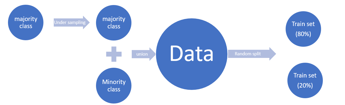
8.4. Unbalanced data: Undersampling¶

Since we use PySpark to deal with the big data, Undersampling for Unbalanced Classification is a useful method to deal with the Unbalanced data. Undersampling is a popular technique for unbalanced datasets to reduce the skew in class distributions. However, it is well-known that undersampling one class modifies the priors of the training set and consequently biases the posterior probabilities of a classifier. After you applied the Undersampling, you need to recalibrate the Probability Calibrating Probability with Undersampling for Unbalanced Classification.

df = spark.createDataFrame([
    (0, "Yes"),
    (1, "Yes"),
    (2, "Yes"),
    (3, "Yes"),
    (4, "No"),
    (5, "No")
], ["id", "label"])
df.show()

+---+-----+
| id|label|
+---+-----+
|  0|  Yes|
|  1|  Yes|
|  2|  Yes|
|  3|  Yes|
|  4|   No|
|  5|   No|
+---+-----+

8.4.1. Calculate undersampling Ratio¶

import math
def round_up(n, decimals=0):
    multiplier = 10 ** decimals
    return math.ceil(n * multiplier) / multiplier

  # drop missing value rows
df = df.dropna()
# under-sampling majority set
label_Y = df.filter(df.label=='Yes')
label_N = df.filter(df.label=='No')
sampleRatio = round_up(label_N.count() / df.count(),2)

8.4.2. Undersampling¶

label_Y_sample = label_Y.sample(False, sampleRatio)
# union minority set and the under-sampling majority set
data = label_N.unionAll(label_Y_sample)
data.show()

+---+-----+
| id|label|
+---+-----+
|  4|   No|
|  5|   No|
|  1|  Yes|
|  2|  Yes|
+---+-----+

8.4.3. Recalibrating Probability¶

Undersampling is a popular technique for unbalanced datasets to reduce the skew in class distributions. However, it is well-known that undersampling one class modifies the priors of the training set and consequently biases the posterior probabilities of a classifier Calibrating Probability with Undersampling for Unbalanced Classification.

predication.withColumn('adj_probability',sampleRatio*F.col('probability')/((sampleRatio-1)*F.col('probability')+1))