Homework #1

You can also get the PDF format of Wenqiang’s Homework.

Required library

library(histogram)
library(plyr)

Load data

homeownership = read.table("./data/ex3-11.TXT", header = T)
hiv = read.table("./data/ex3-76.TXT", header = T)

Q 3.11(a)

## X1985
par(mfrow=c(3,1))
hist(homeownership$X1985, freq = F, right = F, ylim = c(0, 0.12), 
     xlim = c(30, 100), xlab = "1985", ylab = "Relative Frequency", 
     main = "", breaks = 20)
## X1996
hist(homeownership$X1996, freq = F, right = F, ylim = c(0, 0.12), 
     xlim = c(30, 100), xlab = "1996", ylab = "Relative Frequency", 
     main = "", breaks = 20)
## X2002
hist(homeownership$X2002, freq = F, right = F, ylim = c(0, 0.12), 
     xlim = c(30, 100), xlab = "2002", ylab = "Relative Frequency", 
     main = "", breaks = 20)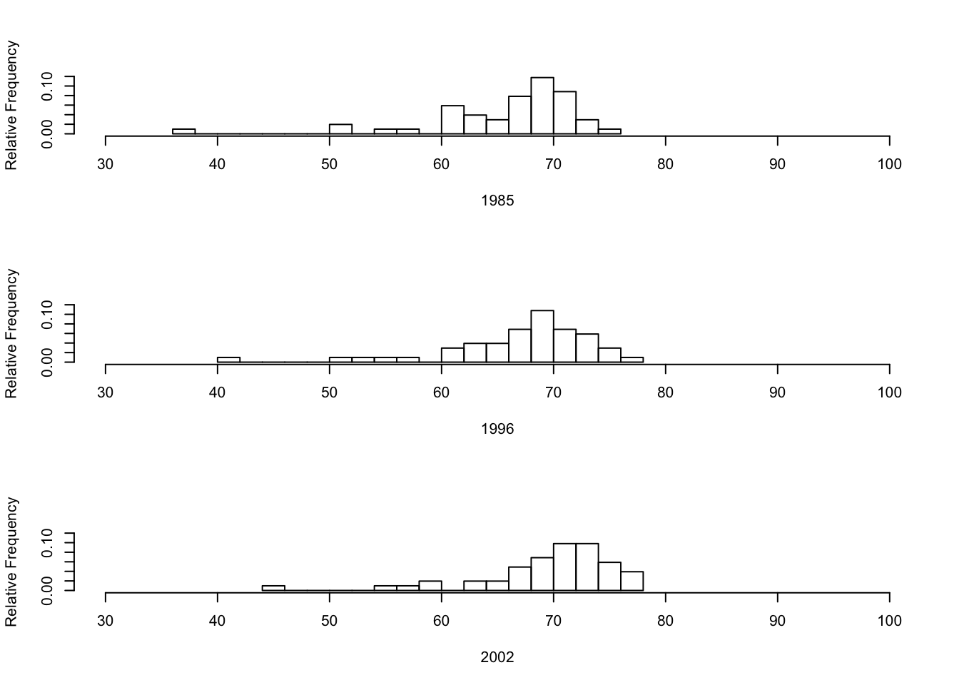

Q 3.11(b)

The three histograms have similar shape. The average homeownship rate has increased since 1985.

colMeans(homeownership[,2:4])

##    X1985    X1996    X2002 
## 65.87647 66.84314 69.44902

Q 3.11(c)

Increases in families incomes so more people can purchase homes.

Q 3.11(d)

The average homeship rate increases from 65.87% to 69.44% from 1985 to 2002. This is very small inscrease in a long time period. The Congress should write laws to increase tax deductions so that more people can purchase homes.

Q 3.12

Stem-and-leaf plots

Year 1985

stem(homeownership$X1985)

## 
##   The decimal point is 1 digit(s) to the right of the |
## 
##   3 | 7
##   4 | 
##   4 | 
##   5 | 014
##   5 | 7
##   6 | 1111122344
##   6 | 5667777888888899999
##   7 | 0000000011122234
##   7 | 6

Year 1996

stem(homeownership$X1996)

## 
##   The decimal point is 1 digit(s) to the right of the |
## 
##   4 | 0
##   4 | 
##   5 | 13
##   5 | 57
##   6 | 1222333
##   6 | 5555777778888888999999
##   7 | 000112233333344
##   7 | 57

Year 2002

stem(homeownership$X2002)

## 
##   The decimal point is 1 digit(s) to the right of the |
## 
##   4 | 4
##   4 | 
##   5 | 
##   5 | 578
##   6 | 034
##   6 | 666777789999
##   7 | 000000000222222333444444
##   7 | 55566777

Q 3.13: Descriptions of the stem-and-leaf plots

Both the stem-and-leaf and histogram for all three years are asymmetrical, unimodal and left skewed.

Q 3.36(a)

Boxplots

boxplot(homeownership$X1985, xlab="1985", ylim=c(30, 80))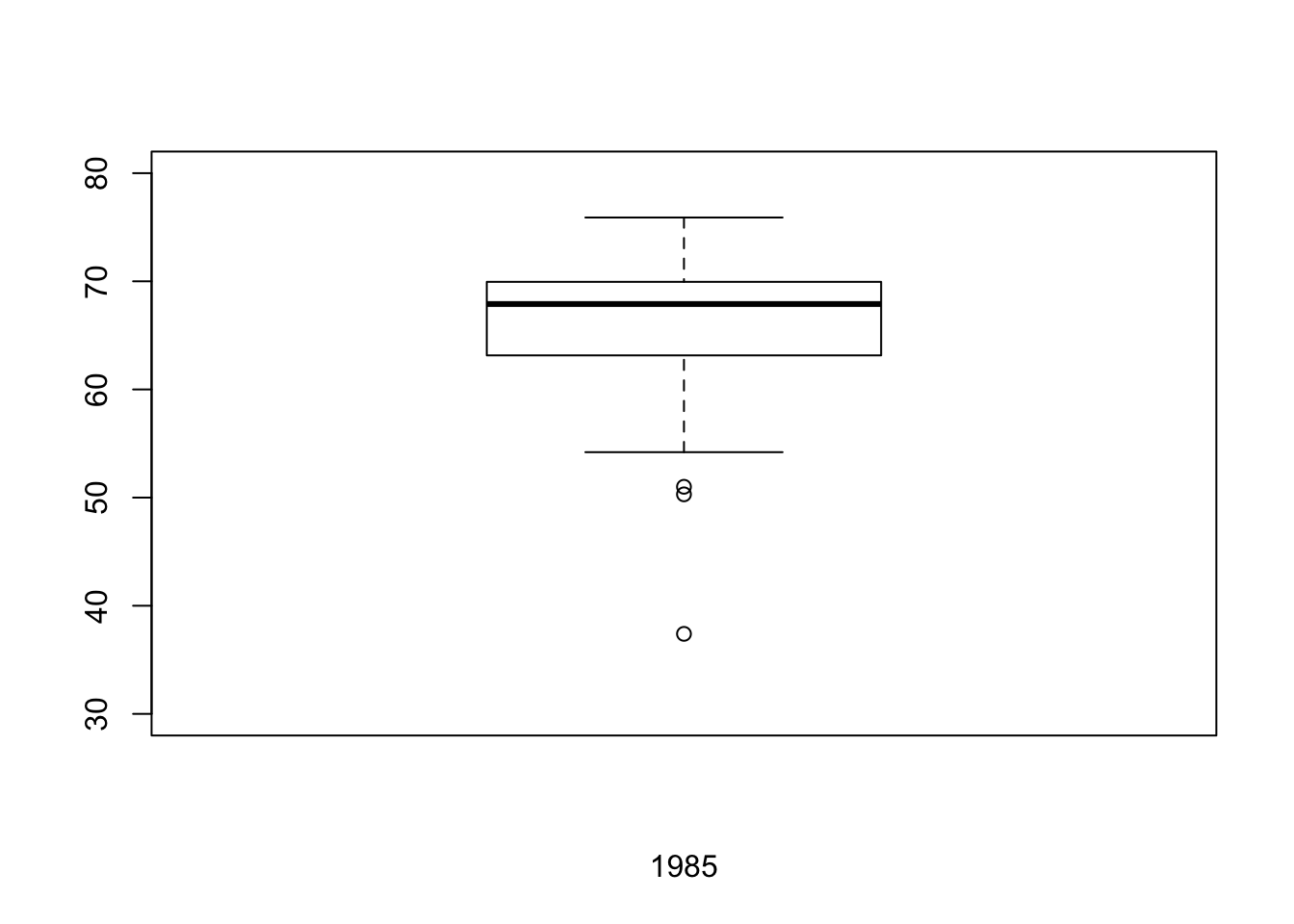

boxplot(homeownership$X1996, xlab="1996", ylim=c(30, 80))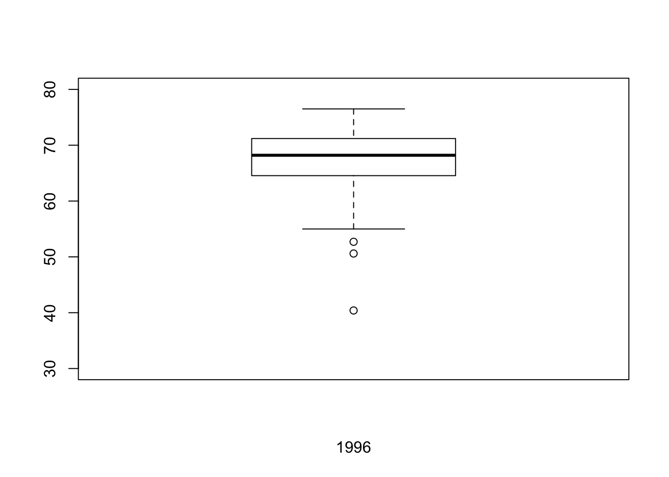

boxplot(homeownership$X2002, xlab="2002", ylim=c(30, 80))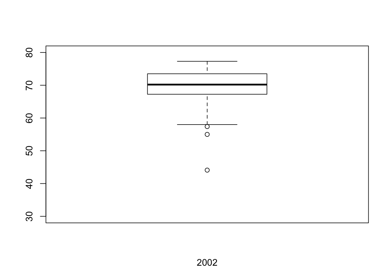

Three boxplots are all asysmmetric and left skewed.

Q 3.36(b)

Boxplots give the same information from the stem-and-leaf and histograms in 3.11: asysmmetric and left skewed data for all three years.

Q 3.37

Mean, median and standard deviation

colMeans(homeownership[,2:4])

##    X1985    X1996    X2002 
## 65.87647 66.84314 69.44902

Median

colwise(median)(homeownership[,2:4])

##   X1985 X1996 X2002
## 1  67.9  68.2  70.2

Standard deviation

colwise(sd)(homeownership[,2:4])

##      X1985    X1996    X2002
## 1 6.734407 6.688027 6.162901

Q 3.37(a)

The median is more approriate than the mean for these data sets, because the data sets are skewed

Q 3.37(b)

The variability continously descreased since 1985.

Q 3.38

y = c(homeownership$X1985, homeownership$X1996, homeownership$X2002)
x = rep(c("X1985", "X1996", "X2002"), each=nrow(homeownership))
boxplot(y~x)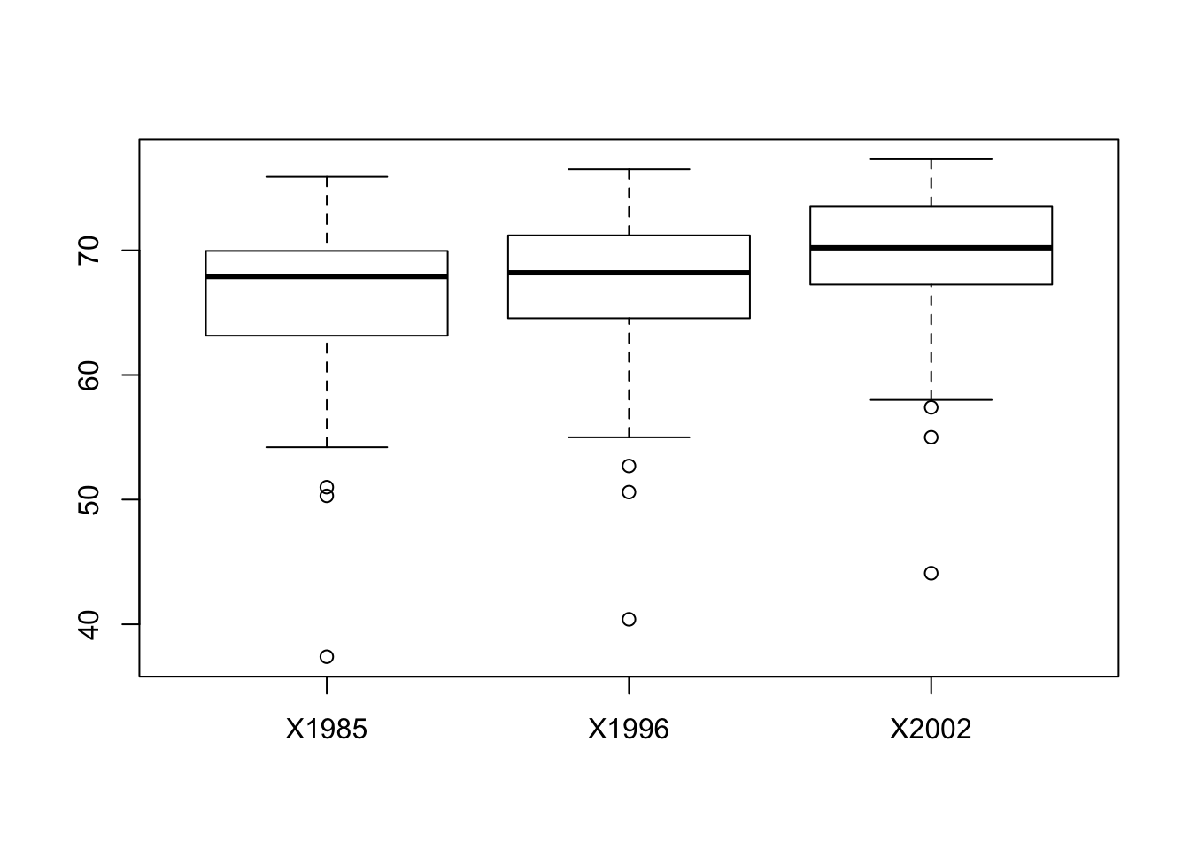

Q 3.38(a)

The median hownownership rate continously increased from 1985 to 2002

Q 3.38(b)

The variation hownownership rate continously decreased from 1985 to 2002.

Q 3.38(c)

Yes.
State 9, 33, 12 are extremely low in homeownership rate in 1985.
State 9, 12, 33 are extremely low in homeownership rate in 1996.
State 9, 33, 12 are extremely low in homeownership rate in 2002.

Q 3.38(d)

No.

3.76(a)

Mean, median and standard deviation

data.frame(mean=mean(hiv$HIV_RNA), 
           median=median(hiv$HIV_RNA),
           std=sd(hiv$HIV_RNA))

##       mean  median      std
## 1 61667.95 13956.5 117539.3

3.76(b)

25%, 50% and 75% percentiles

quantile(hiv$HIV_RNA)[2:4]

##      25%      50%      75% 
##  9967.00 13956.50 56975.75

3.76(c)

boxplot

boxplot(hiv$HIV_RNA, main="HIV RNA")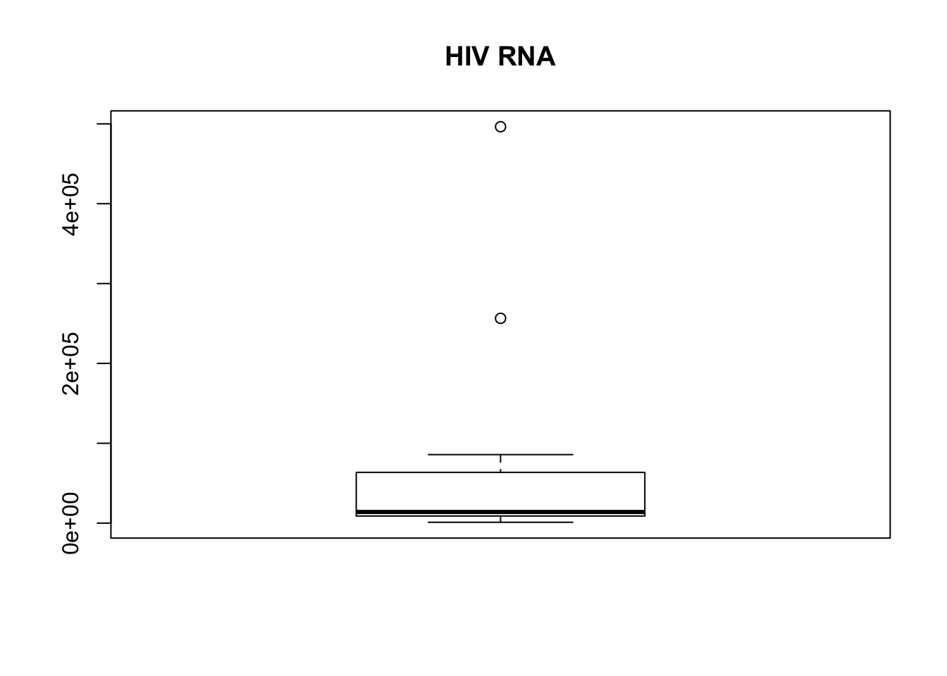

histogram

hist(hiv$HIV_RNA, xlab="HIV RNA", main="", 
     ylim=c(0,20), breaks=10)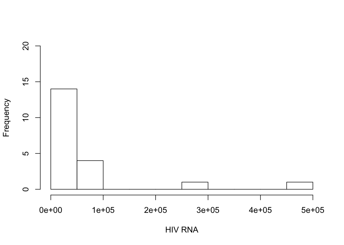

3.76(d)

The distribution is unimodal and right skewed.