Homework #7

Load data

riverValley = read.csv("./data/ArkansasRiverValley.csv")

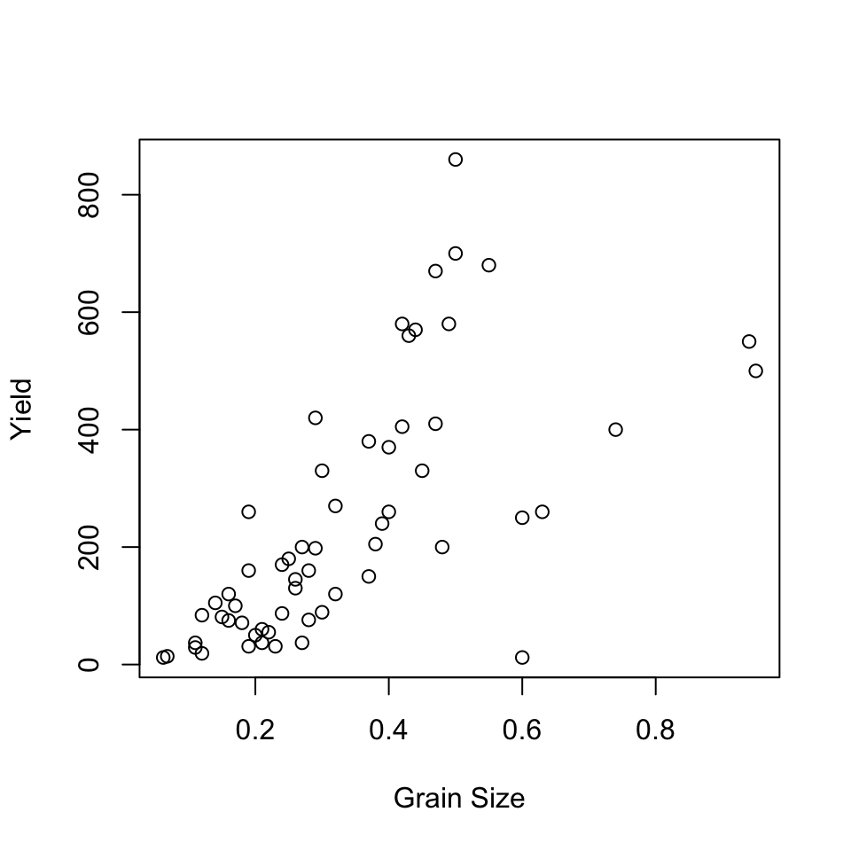
Correlation

• (1). scatterplot

plot(Yield~GrainSize, data=riverValley, xlab="Grain Size", ylab="Yield")

• (2). Compute
  • Pearson \(r = 0.667871\)
  • Spearmans \(\rho\) = 0.7634203

## Pearson's r
cor(riverValley$GrainSize, riverValley$Yield, method="pearson")

## [1] 0.667871

## Spearman's rho
cor(riverValley$GrainSize, riverValley$Yield, method="spearman")

## [1] 0.7634203

• (3). Test hypothesis
  • 1. P value = 7.543e-09 < 0.05, reject \(H_{0}\). There is a significant correlation between grain size and yield.
  • 2. P value = 2.059e-12 < 0.05, reject \(H_{0}\). There is a significant correlation between grain size and yield.

cor.test(riverValley$GrainSize, riverValley$Yield, method="pearson")

## 
##  Pearson's product-moment correlation
## 
## data:  riverValley$GrainSize and riverValley$Yield
## t = 6.7748, df = 57, p-value = 7.543e-09
## alternative hypothesis: true correlation is not equal to 0
## 95 percent confidence interval:
##  0.4967473 0.7890091
## sample estimates:
##      cor 
## 0.667871

cor.test(riverValley$GrainSize, riverValley$Yield, method="spearman")

## 
##  Spearman's rank correlation rho
## 
## data:  riverValley$GrainSize and riverValley$Yield
## S = 8095.8, p-value = 2.059e-12
## alternative hypothesis: true rho is not equal to 0
## sample estimates:
##       rho 
## 0.7634203

• (4). 95% confidence interval for \(\rho\) = [0.630624, 0.8527845]

library(mada)

## Loading required package: ellipse

## 
## Attaching package: 'ellipse'

## The following object is masked from 'package:car':
## 
##     ellipse

## Loading required package: mvmeta

## This is mvmeta 0.4.7. For an overview type: help('mvmeta-package').

rho = cor.test(riverValley$GrainSize, riverValley$Yield, method="spearman")$estimate
CIrho(rho, dim(riverValley)[1])

##            rho    2.5 %    97.5 %
## [1,] 0.7634203 0.630624 0.8527845

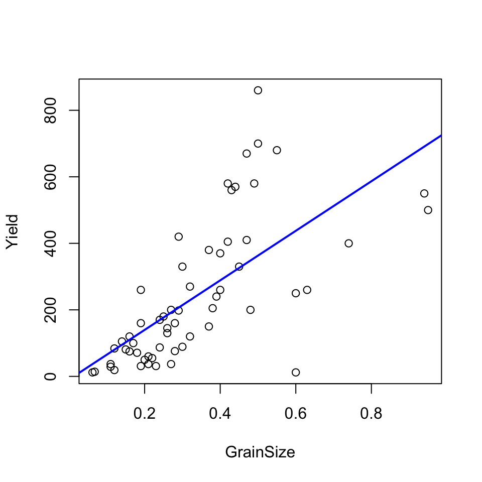
Regression

• (1). Scatterplot

rivervalley.lmfit = lm(Yield~GrainSize, data=riverValley)
plot(Yield~GrainSize, data=riverValley)
abline(rivervalley.lmfit, col="blue", lwd=2)

• (2). Estimates
  • \(\beta_{0} = -9.294\)
  • \(\beta_{1} = 744.979\)

rivervalley.lmfit

## 
## Call:
## lm(formula = Yield ~ GrainSize, data = riverValley)
## 
## Coefficients:
## (Intercept)    GrainSize  
##      -9.294      744.979

• (3). Test the hypothesis
  • p value = 7.54e-09 < 0.05, reject \(H_{0}\)

summary(rivervalley.lmfit)

## 
## Call:
## lm(formula = Yield ~ GrainSize, data = riverValley)
## 
## Residuals:
##     Min      1Q  Median      3Q     Max 
## -425.69 -100.43  -28.70   55.03  496.80 
## 
## Coefficients:
##             Estimate Std. Error t value Pr(>|t|)    
## (Intercept)   -9.294     42.255  -0.220    0.827    
## GrainSize    744.979    109.964   6.775 7.54e-09 ***
## ---
## Signif. codes:  0 '***' 0.001 '**' 0.01 '*' 0.05 '.' 0.1 ' ' 1
## 
## Residual standard error: 159.4 on 57 degrees of freedom
## Multiple R-squared:  0.4461, Adjusted R-squared:  0.4363 
## F-statistic:  45.9 on 1 and 57 DF,  p-value: 7.543e-09

• 4. Residuals

res = rivervalley.lmfit$residuals
fitted = rivervalley.lmfit$fitted.values
y = riverValley$Yield
data.frame(Y=y, Fitted_value = fitted, Residuals = res)

##      Y Fitted_value    Residuals
## 1   12     36.89486  -24.8948554
## 2   14     41.36473  -27.3647300
## 3   29     72.65385  -43.6538518
## 4   37     72.65385  -35.6538518
## 5   19     80.10364  -61.1036427
## 6   84     80.10364    3.8963573
## 7  105     95.00322    9.9967755
## 8   81    102.45302  -21.4530154
## 9   75    109.90281  -34.9028063
## 10 120    109.90281   10.0971937
## 11 100    117.35260  -17.3525972
## 12  71    124.80239  -53.8023882
## 13  31    132.25218 -101.2521791
## 14 160    132.25218   27.7478209
## 15 260    132.25218  127.7478209
## 16  50    139.70197  -89.7019700
## 17  37    147.15176 -110.1517609
## 18  60    147.15176  -87.1517609
## 19  55    154.60155  -99.6015518
## 20  31    162.05134 -131.0513427
## 21  87    169.50113  -82.5011336
## 22 170    169.50113    0.4988664
## 23 180    176.95092    3.0490755
## 24 130    184.40072  -54.4007154
## 25 145    184.40072  -39.4007154
## 26  37    191.85051 -154.8505063
## 27 200    191.85051    8.1494937
## 28  76    199.30030 -123.3002972
## 29 160    199.30030  -39.3002972
## 30 198    206.75009   -8.7500881
## 31  89    214.19988 -125.1998790
## 32 420    206.75009  213.2499119
## 33 330    214.19988  115.8001210
## 34 120    229.09946 -109.0994609
## 35 270    229.09946   40.9005391
## 36 150    266.34842 -116.3484154
## 37 380    266.34842  113.6515846
## 38 205    273.79821  -68.7982063
## 39 240    281.24800  -41.2479972
## 40 260    288.69779  -28.6977881
## 41 370    288.69779   81.3022119
## 42 405    303.59737  101.4026301
## 43 580    303.59737  276.4026301
## 44 560    311.04716  248.9528391
## 45 570    318.49695  251.5030482
## 46 330    325.94674    4.0532573
## 47 410    340.84632   69.1536755
## 48 670    340.84632  329.1536755
## 49 200    348.29612 -148.2961154
## 50 580    355.74591  224.2540937
## 51 700    363.19570  336.8043028
## 52 860    363.19570  496.8043028
## 53 680    400.44465  279.5553483
## 54  12    437.69361 -425.6936063
## 55 250    437.69361 -187.6936063
## 56 260    460.04298 -200.0429790
## 57 400    541.99068 -141.9906790
## 58 550    690.98650 -140.9864972
## 59 500    698.43629 -198.4362881