Homework #4
Ming Chen & Wenqiang Feng
2/2/2017
You can also get the PDF format of Wenqiang’s Homework.
Q 5.66
Q 5.66(a)
- Evaluate whether the sample is from a normal distribution
- From the normal quantile plot, we can see that the data points appear to be realtively close to the fitted line, which suggests that the normality of the population is plausible.
dissolution = c(19.5,19.7,19.7,20.4,19.2,19.5,19.6,20.8,19.9,
                19.2,20.1,19.8,20.4,19.8,19.6,19.5,19.3,19.7,
                19.5,20.6,20.4,19.9,20.0,19.8)
qqnorm(dissolution)
qqline(dissolution)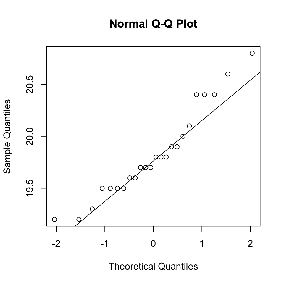
Q 5.66(b)
- Mean =
mean(dissolution)= 19.8291667 - The 99% CI for unknown \(\mu\) and \(\sigma\) is given by \(\bar{y} \pm t_{\alpha/2}s/\sqrt{n}\), where
- \(\bar{y}\) =
mean(dissolution)= 19.8291667 - \(t_{\alpha/2}\) = \(t_{0.01/2, df=23}\) = 2.8073357
- s = 0.4318607
- n = 24
- \(\bar{y}\) =
- so, 99% CI = \(19.83 \pm 2.81(0.432)\sqrt{23}\) = [19.58, 20.08]
Q 5.66(c)
- Let \(H_{0} = \mu\geq\mu_{0}, H_{a} = \mu<\mu_{0}\). Reject \(H_{0}\) if \(t\geq t_{\alpha}\)
- From the right-tailed t-test, p-value = 0.0325 > 0.01, given that \(\alpha = 0.01\)
- Conclusion: we cann’t reject the \(H_{0}\) hypothesis
t.test(dissolution, mu=20, alternative = "less", conf.level = 0.99)##
## One Sample t-test
##
## data: dissolution
## t = -1.9379, df = 23, p-value = 0.0325
## alternative hypothesis: true mean is less than 20
## 99 percent confidence interval:
## -Inf 20.04954
## sample estimates:
## mean of x
## 19.82917Q 5.68
- Let \(H_{0} = \mu\leq\mu_{0}, H_{a} = \mu>\mu_{0}\). Reject \(H_{0}\) if \(t\geq t_{\alpha}\)
- From the right-tailed t-test, p-value = 0.1485 > 0.05, given that \(\alpha = 0.05\)
- Conclusion: we can’t reject the \(H_{0}\) hypothesis
time = c(28,25,27,31,10,26,30,15,55,12,24,32,28,42,38)
t.test(time, mu=25, alternative = "greater")
##
## One Sample t-test
##
## data: time
## t = 1.0833, df = 14, p-value = 0.1485
## alternative hypothesis: true mean is greater than 25
## 95 percent confidence interval:
## 22.99721 Inf
## sample estimates:
## mean of x
## 28.2Q 5.72
Q 5.72(a)
- 95% CI: [26.26906, 34.75951]
- Explanation: randomely select a healthy army inductee, the probablity that his exercise capacity will fall into [26.26906, 34.75951] is 95%.
capacities = c(23,19,36,12,41,43,19,28,14,44,15,46,36,25,
               35,25,29,17,51,33,47,42,45,23,29,18,14,48,
               21,49,27,39,44,18,13)
CI95 = t.test(capacities)$conf.int
CI95
## [1] 26.26906 34.75951
## attr(,"conf.level")
## [1] 0.95Q 5.72(b)
- 99% CI: [24.81485, 36.21372]
- The 99% confidence interval becomes wider than 95% confidence interval
CI99 = t.test(capacities, conf.level=0.99)$conf.int
CI99
## [1] 24.81485 36.21372
## attr(,"conf.level")
## [1] 0.99