Homework #5
Ming Chen & Wenqiang Feng
2/2/2017
You can also get the PDF format of Wenqiang’s Homework.
Exercise 6.44
- (a). What are the populations of interest?
- The plants of tobacco treated with two different fumigants
- The variable being studies is the number of parasites from the plants
- (b). Yes. The p-value is 2.089e-05, which is a strong evidence to indicate a difference in the mean level of parasites for the two fumigants.
F1 = c(77,40,11,31,28,50,53,26,33)
F2 = c(76,38,10,29,27,48,51,24,32)

t.test(F1, F2, paired = T, conf.level = 0.90)
##
## Paired t-test
##
## data: F1 and F2
## t = 8.8544, df = 8, p-value = 2.089e-05
## alternative hypothesis: true difference in means is not equal to 0
## 90 percent confidence interval:
## 1.228866 1.882245
## sample estimates:
## mean of the differences
## 1.555556- (c). the size of diference = 1.555556, 90% CI = [1.228866, 1.882245]
Exercise 6.46
abundance = c(5124,2904,3600,2880,2578,4146,1048,1336,394,7370,6762,744,1874,
              3228,2032,3256,3816,2438,4897,1346,1676,2008,2224,1234,1598,2182)
depth = c(rep(40, 13), rep(100, 13))
oil_traj = c(rep(c("within", "outside"), c(7,6)),
             rep(c("within", "outside"), c(7,6)))
pop_abundance = data.frame(abundance, as.factor(depth), oil_traj)library(dplyr)##
## Attaching package: 'dplyr'## The following object is masked from 'package:gridExtra':
##
## combine## The following object is masked from 'package:MASS':
##
## select## The following objects are masked from 'package:plyr':
##
## arrange, count, desc, failwith, id, mutate, rename, summarise,
## summarize## The following objects are masked from 'package:stats':
##
## filter, lag## The following objects are masked from 'package:base':
##
## intersect, setdiff, setequal, unionwithin = filter(pop_abundance, oil_traj=='within')$abundance
outside = filter(pop_abundance, oil_traj=='outside')$abundanceExercise 6.46 (a)
- Since the variances between the two groups are very different, we use the separate variance t-test.
- \(Var_{within}\) =
var(within)= 1.419065210^{6} - \(Var_{outside}\) =
var(outside)= 4.966544310^{6}
- \(Var_{within}\) =
- separate variance t-test
- \(H_{0}: \mu_{within} = \mu_{outside}\) vs. \(H_{a}: \mu_{within} \neq \mu_{outside}\)
- P-value = 0.384 > 0.05, fail to rejct the \(H_{0}\)
- Conclusion: no sufficient evidence to indicate a difference in average population abundance
t.test(within, outside, var.equal = FALSE)##
## Welch Two Sample t-test
##
## data: within and outside
## t = 0.89466, df = 16.224, p-value = 0.384
## alternative hypothesis: true difference in means is not equal to 0
## 95 percent confidence interval:
## -877.7749 2162.1558
## sample estimates:
## mean of x mean of y
## 3092.357 2450.167Exercise 6.46 (b)
- Size of the difference: 0
- 95% CI: [-877.7749, 2162.1558]
Exercise 6.46 (c)
- Required conditions:
- independent samples
- two samples are approximately normally distributed
Exercise 6.46 (d)
- QQ plot shows that
- the data from the within oil trajectory appears normally distributed
- the data from the outside oil trajectory is not normally distributed
par(mfcol=c(1,2))
qqnorm(within, main="Within oil trajectory")
qqline(within)

qqnorm(outside, main="Outside oil trajectory")
qqline(outside)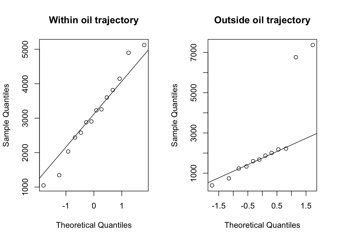
- Unequal variance
- The two samples have unequal variances
- Outside oil trajectory data has larger variance
par(mfcol=c(1,1))
boxplot(within, outside, names=c("within", "outside"))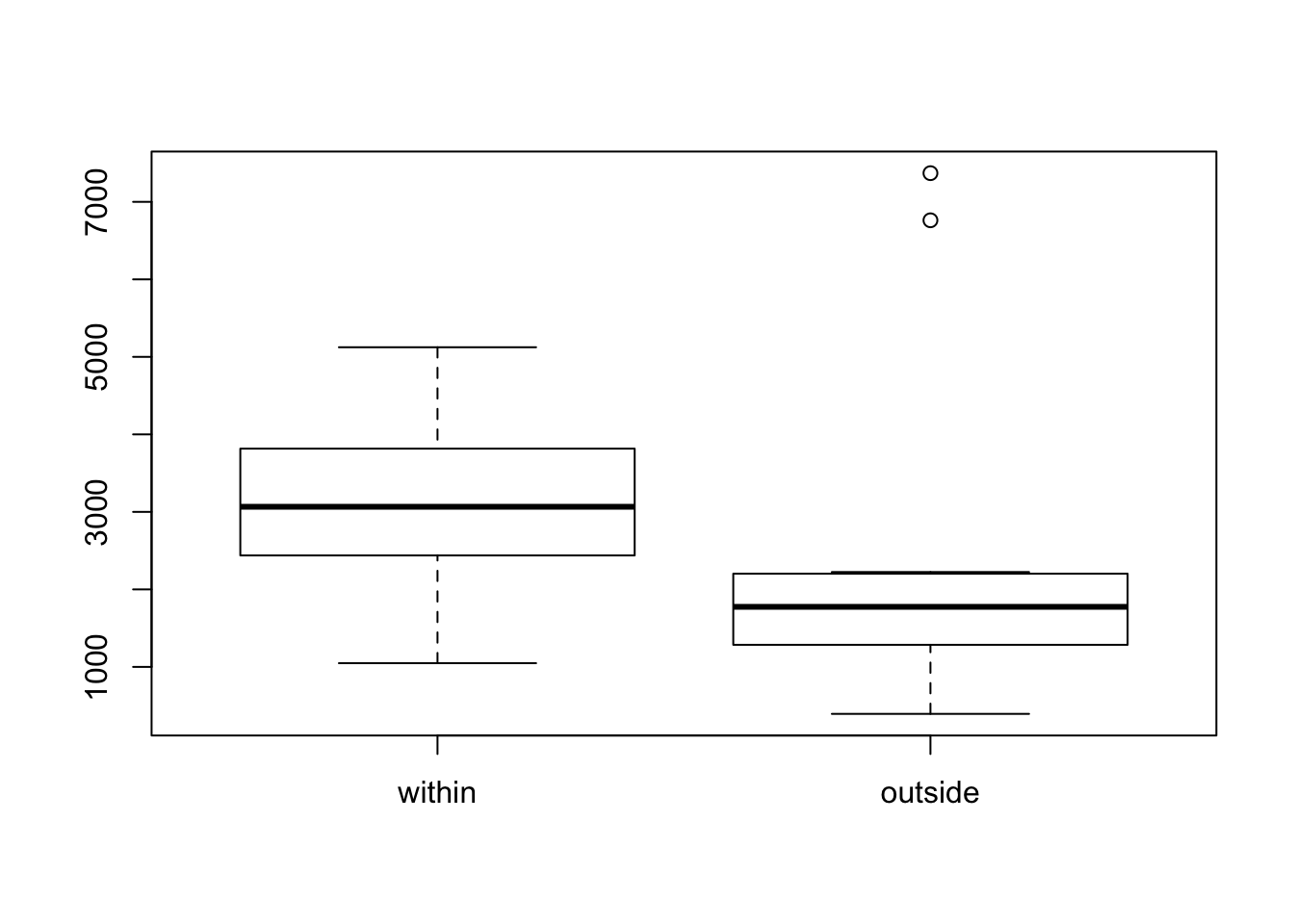
Exercise 7.25(a)
- Data input
portfolio1 = c(130,135,135,131,129,135,126,136,127,132)
portfolio2 = c(154,144,147,150,155,153,149,139,140,141)
sd(portfolio1)^2
## [1] 12.93333- Levene test
- The p-value = 0.07724 > 0.05 from the levene test below indicates that we failed to reject the \(H_{0}\) hypothesis. There is no strong evidence to support that portfolio 2 has higher risk than portfolio 1.
library(car)##
## Attaching package: 'car'## The following object is masked from 'package:dplyr':
##
## recode## The following objects are masked from 'package:HH':
##
## logit, vifdt = data.frame(y=c(portfolio1, portfolio2),
group=rep(c("1", "2"), c(length(portfolio1), length(portfolio2))))
leveneTest(y~group, dt)## Levene's Test for Homogeneity of Variance (center = median)
## Df F value Pr(>F)
## group 1 3.5122 0.07724 .
## 18
## ---
## Signif. codes: 0 '***' 0.001 '**' 0.01 '*' 0.05 '.' 0.1 ' ' 1Exercise 7.26
- Tests for two population variances
- $H_{0}: two variances are eqaul vs. H_{a}: two varainces are not equal
- P-value = 0.1485 > 0.05, fail to rejct \(H_{O}\).
- Conclusion: the two variances are equal
var.test(portfolio1, portfolio2)##
## F test to compare two variances
##
## data: portfolio1 and portfolio2
## F = 0.36421, num df = 9, denom df = 9, p-value = 0.1485
## alternative hypothesis: true ratio of variances is not equal to 1
## 95 percent confidence interval:
## 0.09046343 1.46628824
## sample estimates:
## ratio of variances
## 0.3642053- Tests for normality
- QQ plots show that the two samples are approximately normally distributed.
par(mfcol=c(1,2))
qqnorm(portfolio1, main = "Portfolio 1")
qqline(portfolio1)

qqnorm(portfolio2, main = "Portfolio 2")
qqline(portfolio2)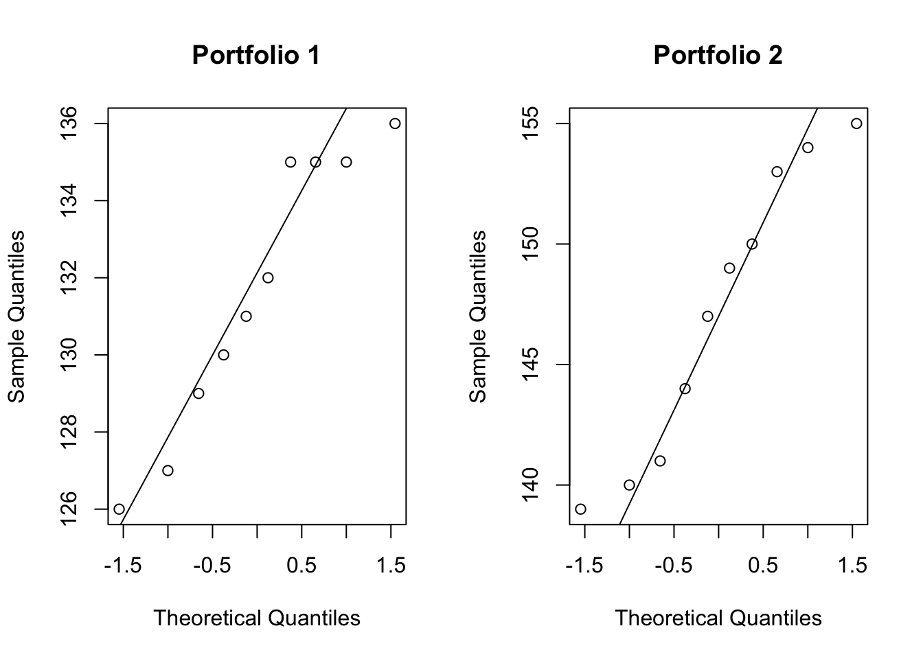
par(mfcol=c(1,1))Since the two samples are randomly selected, normally distributed and have equal variance, I choose the pooled variance t-test to detect if there is any differences in the average returns for the two portfolios.
- \(H_{0}: \mu_{1} = \mu_{2}\) vs. \(H_{a}: \mu_{1} \neq \mu_{2}\)
- P-value = 1.314e-06 < 0.0001, reject \(H_{0}\)
- Conclusion: there is strong evidence that a difference in the mean returns of the two portfolios exits.
t.test(portfolio1, portfolio2, var.equal = T)##
## Two Sample t-test
##
## data: portfolio1 and portfolio2
## t = -7.0877, df = 18, p-value = 1.314e-06
## alternative hypothesis: true difference in means is not equal to 0
## 95 percent confidence interval:
## -20.22415 -10.97585
## sample estimates:
## mean of x mean of y
## 131.6 147.2