Homework #8

Load data

uri = paste0("./data/ex8-32.TXT")
hw8data = read.table(uri, header = T)
attach(hw8data)
hw8data=data.frame(value=c(A,B,C,D), group=rep(LETTERS[1:4], each=length(A)))

Analysis

(1). Hypothesis test
- P value = 5.85e-05, reject \(H_{0}\)
- Conclusion: not all means are equal among the four groups.

hw8data.aov = aov(value~group, hw8data)
summary(hw8data.aov)

##             Df Sum Sq Mean Sq F value   Pr(>F)    
## group        3  6.621  2.2070   11.05 5.85e-05 ***
## Residuals   28  5.594  0.1998                     
## ---
## Signif. codes:  0 '***' 0.001 '**' 0.01 '*' 0.05 '.' 0.1 ' ' 1

(2). Levene’s test
- P value = 0.6428
- The assumption of homegeneity of variance among the four groups is appropriate.

library(car)
leveneTest(value~group, data=hw8data)

## Levene's Test for Homogeneity of Variance (center = median)
##       Df F value Pr(>F)
## group  3  0.5647 0.6428
##       28

(3). Check residuals

The normal QQ plot indicates a normal distribution fits the residuals well.

plot(hw8data.aov, which=2)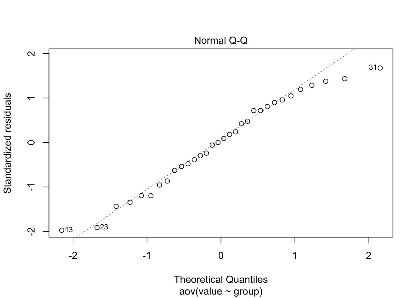

(4). Significantly different groups based on Tukey’s HSD test
- A-B, A-C, B-D, B-D
- Group C has the highest average; Group D has the lowest average.
- No significant difference between group A and D
- No significant difference between group B and C

TukeyHSD(hw8data.aov)

##   Tukey multiple comparisons of means
##     95% family-wise confidence level
## 
## Fit: aov(formula = value ~ group, data = hw8data)
## 
## $group
##        diff         lwr        upr     p adj
## B-A  0.6625  0.05232456  1.2726754 0.0294781
## C-A  0.9375  0.32732456  1.5476754 0.0013447
## D-A -0.1625 -0.77267544  0.4476754 0.8854051
## C-B  0.2750 -0.33517544  0.8851754 0.6132192
## D-B -0.8250 -1.43517544 -0.2148246 0.0049860
## D-C -1.1000 -1.71017544 -0.4898246 0.0001916

plot(value~group, data=hw8data)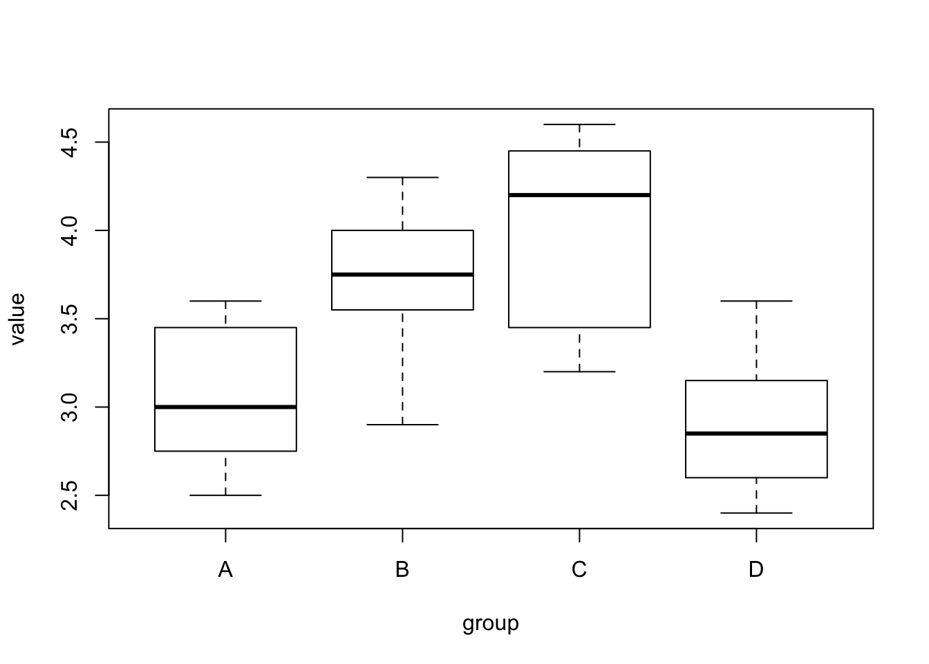

(5). Kruskal-Wallis test
- P value = 0.0008698
- Conclusion: at least two of these four groups have different distributions.

kruskal.test(value~group, data=hw8data)

## 
##  Kruskal-Wallis rank sum test
## 
## data:  value by group
## Kruskal-Wallis chi-squared = 16.561, df = 3, p-value = 0.0008698

Homework #8

Ming Chen & Wenqiang Feng

2/2/2017

You can also get the PDF format of Wenqiang’s Homework.

Load data

Analysis