Load data
weight = read.table("./data/Weight.txt", header =T)
wlabor = read.csv("./data/WLabor.csv", header = T)[,1:3]
potencies = unlist(read.table("./data/Potencies.txt"))
Problem 1
a. Create a stem-and-leaf plot for these data
stem(potencies)
##
##   The decimal point is at the |
##
##   22 | 79
##   23 | 0234
##   23 | 68
##   24 | 013
##   24 | 589
##   25 | 0244
##   25 | 89
##   26 | 144
##   26 | 7799
##   27 | 123
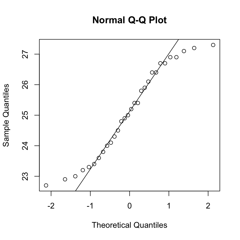
b. Assess the normality of these data
- The shapiro wilk test indicates the data is from a normal distribution.
shapiro.test(potencies)
##
##  Shapiro-Wilk normality test
##
## data:  potencies
## W = 0.93847, p-value = 0.08275
qqnorm(potencies)
qqline(potencies)
c. Provide a 99% confidence interval for the average potency
mu = mean(potencies)
s = sd(potencies)
n = length(potencies)
SE = s/sqrt(n); SE
## [1] 0.2682203
lower = mu - qt(0.995, df=n-1)*SE; lower
## [1] 24.35735
upper = mu + qt(0.995, df=n-1)*SE; upper
## [1] 25.83599
- 99% confidence interval: \([\mu - t_{0.01/2}\frac{s}{\sqrt{n}}, \mu + t_{0.01/2}\frac{s}{\sqrt{n}}]\) = [24.3573479, 25.8359854]
- \(\mu\) = 25.0966667
- s = 1.4691033
- n = 30
- \(t_{0.01/2}\) = 2.7563859
d. Based on your results for part(c), can we conclude that the average potency is 25 mg as advertised?
- Yes. 25 is within the 99% confidence interval [24.35735, 25.83599].
Problem 2
a. Compute the difference scores between percentages for each year and create a stem-and-leaf plot for these difference scores.
library(plyr)
difference_scores = mutate(wlabor, difference_scores = Year_68 - Year_72)
difference_scores
##             City Year_68 Year_72 difference_scores
## 1           N.Y.    0.42    0.45             -0.03
## 2           L.A.    0.50    0.50              0.00
## 3        Chicago    0.52    0.52              0.00
## 4   Philadelphia    0.45    0.45              0.00
## 5        Detroit    0.43    0.46             -0.03
## 6  San Francisco    0.55    0.55              0.00
## 7         Boston    0.45    0.60             -0.15
## 8          Pitt.    0.34    0.49             -0.15
## 9      St. Louis    0.45    0.35              0.10
## 10   Connecticut    0.54    0.55             -0.01
## 11   Wash., D.C.    0.42    0.52             -0.10
## 12         Cinn.    0.51    0.53             -0.02
## 13     Baltimore    0.49    0.57             -0.08
## 14        Newark    0.54    0.53              0.01
## 15 Minn/St. Paul    0.50    0.59             -0.09
## 16       Buffalo    0.58    0.64             -0.06
## 17       Houston    0.49    0.50             -0.01
## 18     Patterson    0.56    0.57             -0.01
## 19        Dallas    0.63    0.64             -0.01
- Stem-and-leaf plot for difference scores
stem(difference_scores$difference_scores)
##
##   The decimal point is 1 digit(s) to the left of the |
##
##   -1 | 550
##   -0 | 9863321111
##    0 | 00001
##    1 | 0
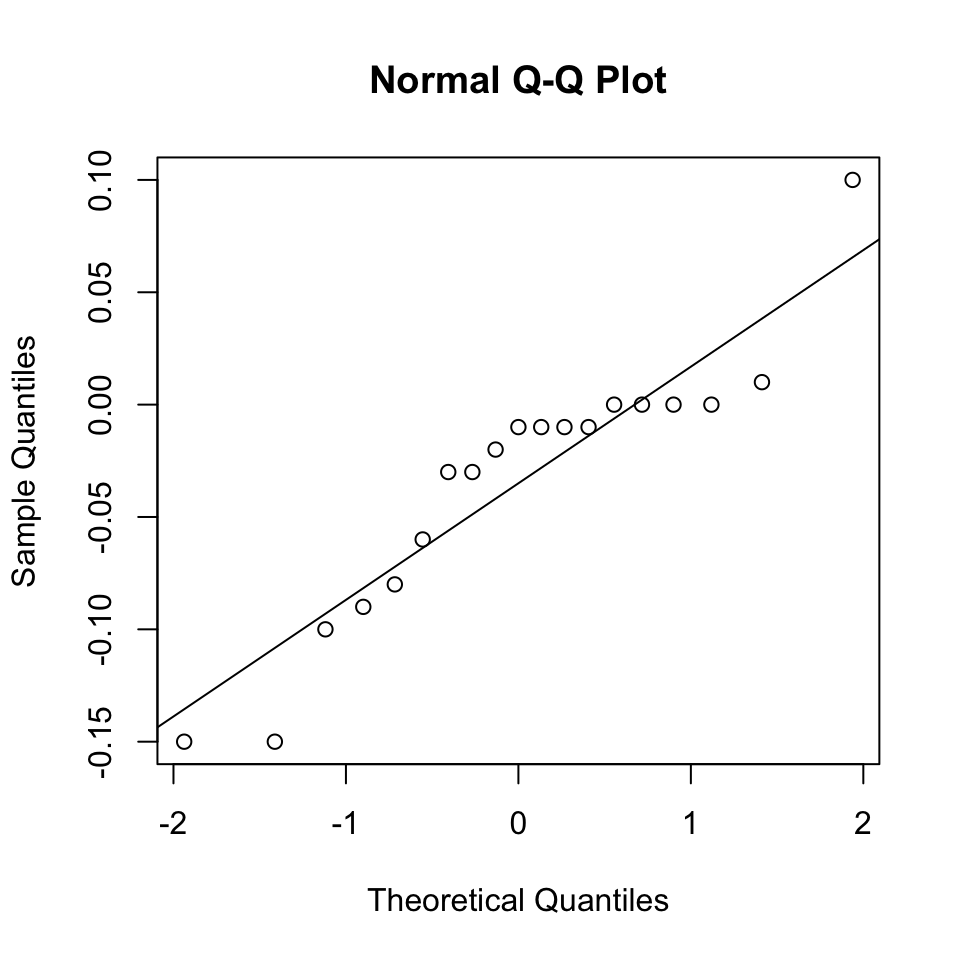
b. Assess the normality of these difference scores.
- The shapiro wilk test indicates non-normality of these differenct scores
shapiro.test(difference_scores$difference_scores)
##
##  Shapiro-Wilk normality test
##
## data:  difference_scores$difference_scores
## W = 0.89814, p-value = 0.04503
qqnorm(difference_scores$difference_scores)
qqline(difference_scores$difference_scores)
c. Based upon the results from part(b), wilcoxon signed ranks test is applied to determined whether there is a significant difference.
- P value = 0.01324 < 0.05, indicates a significant difference between the average percentages in 1968 and in 1972.
wilcoxTest = wilcox.test(difference_scores$difference_scores, conf.int = T); wilcoxTest
##
##  Wilcoxon signed rank test with continuity correction
##
## data:  difference_scores$difference_scores
## V = 16, p-value = 0.01324
## alternative hypothesis: true location is not equal to 0
## 95 percent confidence interval:
##  -0.08004133 -0.01002685
## sample estimates:
## (pseudo)median
##    -0.04498224
d. Estimate the difference with a 95% condifence interval
difference = wilcoxTest$estimate; difference
## (pseudo)median
##    -0.04498224
CI95 = as.numeric(wilcoxTest$conf.int); CI95
## [1] -0.08004133 -0.01002685
- Difference = -0.0449822
- 95% CI = -0.0800413, -0.0100269
Problem 3
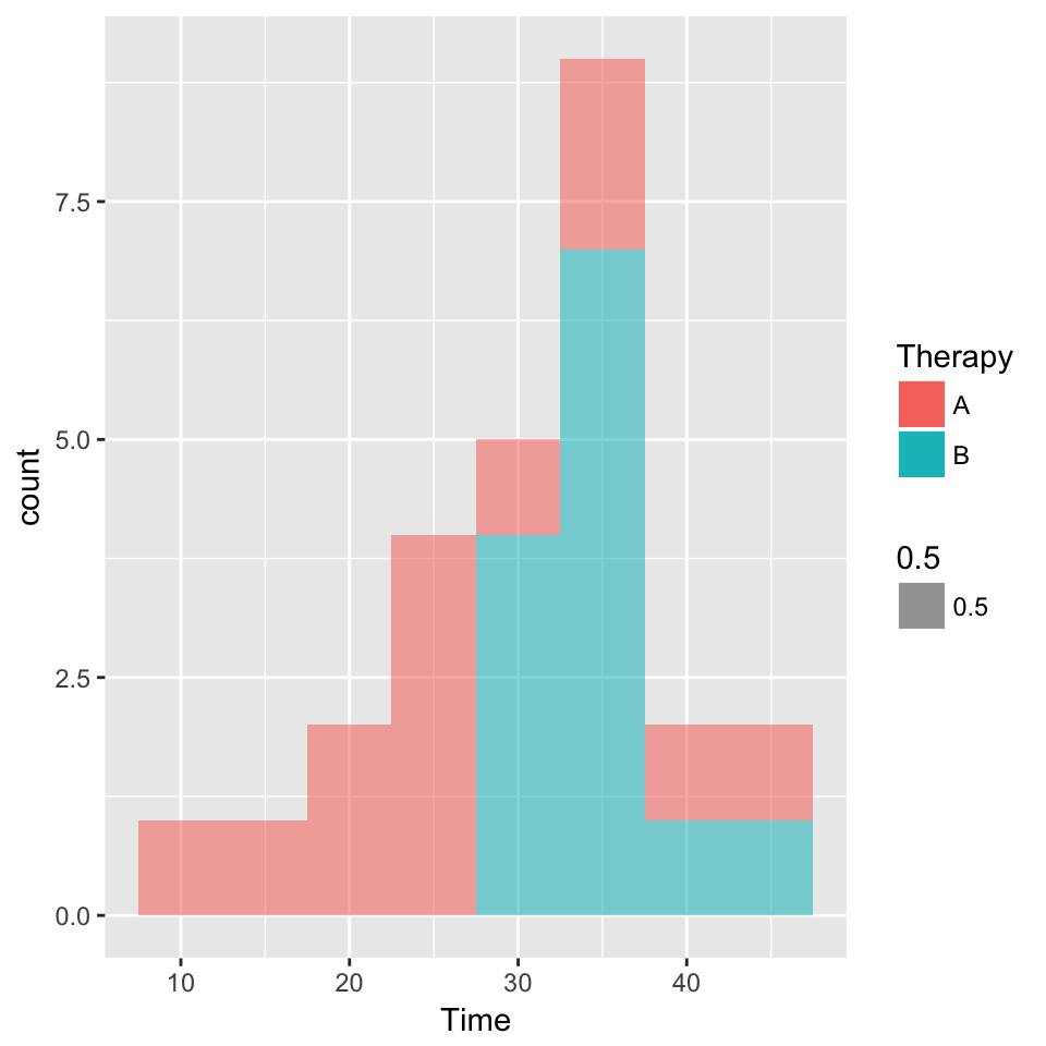
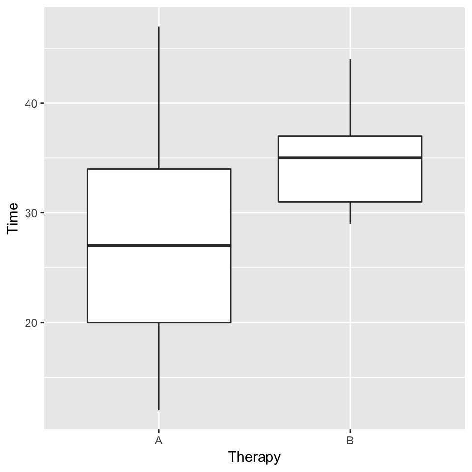
a. Stacked histogram and side-by-side box-and-whisker plots
library(ggplot2)
ggplot(weight, aes(Time, fill=Therapy, alpha=0.5)) +
  geom_histogram(binwidth = 5)
ggplot(weight, aes(Therapy, Time)) +
  geom_boxplot()
b. Assess the normality of data from each of the two therapies
- Normality assessment for therapy A
- p value = 0.7462, indicating that the data is from a normal distribution.
therapyA = weight[weight$Therapy=="A", 2]
shapiro.test(therapyA)
##
##  Shapiro-Wilk normality test
##
## data:  therapyA
## W = 0.95952, p-value = 0.7462
- Normality assessment for therapy B
- p value = 0.4024, indicating that the data is from a normal distribution.
therapyB = weight[weight$Therapy=="B", 2]
shapiro.test(therapyB)
##
##  Shapiro-Wilk normality test
##
## data:  therapyB
## W = 0.93559, p-value = 0.4024
c. 95% confidence interval for the mean times
mu = mean(therapyA)
s = sd(therapyA)
n = length(therapyA)
SE = s/sqrt(n); SE
## [1] 2.725799
lower = mu - qt(0.975, df=n-1)*SE; lower
## [1] 21.67638
upper = mu + qt(0.975, df=n-1)*SE; upper
## [1] 33.55439
- 95% confidence interval for therapy A
- 99% confidence interval: \([\mu - t_{0.05/2}\frac{s}{\sqrt{n}}, \mu + t_{0.01/2}\frac{s}{\sqrt{n}}]\) = [21.6763787, 33.5543905]
- \(\mu\) = 27.6153846
- s = 9.8280081
- n = 13
- \(t_{0.05/2}\) = 2.1788128
mu = mean(therapyB)
s = sd(therapyB)
n = length(therapyB)
SE = s/sqrt(n); SE
## [1] 1.117372
lower = mu - qt(0.975, df=n-1)*SE; lower
## [1] 32.25776
upper = mu + qt(0.975, df=n-1)*SE; upper
## [1] 37.12685
- 95% confidence interval for therapy B
- 99% confidence interval: \([\mu - t_{0.05/2}\frac{s}{\sqrt{n}}, \mu + t_{0.01/2}\frac{s}{\sqrt{n}}]\) = [32.2577627, 37.1268527]
- \(\mu\) = 34.6923077
- s = 4.0287429
- n = 13
- \(t_{0.05/2}\) = 2.1788128
d. Determine if the variances of the times from the two therapies are equal
varTest=var.test(therapyA, therapyB); varTest
##
##  F test to compare two variances
##
## data:  therapyA and therapyB
## F = 5.951, num df = 12, denom df = 12, p-value = 0.00426
## alternative hypothesis: true ratio of variances is not equal to 1
## 95 percent confidence interval:
##   1.815845 19.503164
## sample estimates:
## ratio of variances
##           5.951027
- p value = 0.0042603 < 0.05, reject \(H_{0}\). The variances are not equal.
e. Test whether the means of the times of the two therapies are equal
- Based upon the results from part(d), wilcox rank sum test is applied.
wilcoxTest=wilcox.test(therapyA, therapyB, conf.int = T); wilcoxTest
## Warning in wilcox.test.default(therapyA, therapyB, conf.int = T): cannot
## compute exact p-value with ties
## Warning in wilcox.test.default(therapyA, therapyB, conf.int = T): cannot
## compute exact confidence intervals with ties
##
##  Wilcoxon rank sum test with continuity correction
##
## data:  therapyA and therapyB
## W = 35, p-value = 0.01185
## alternative hypothesis: true location shift is not equal to 0
## 95 percent confidence interval:
##  -13.999970  -2.000003
## sample estimates:
## difference in location
##              -8.000047
- p value = 0.0118461, indicating a significant difference in the means of the times of the two therapies.
difference = wilcoxTest$estimate; difference
## difference in location
##              -8.000047
CI95 = as.numeric(wilcoxTest$conf.int); CI95
## [1] -13.999970 -2.000003
- Time difference = -8.0000465
- 95% confidence interval = -13.9999697, -2.0000026
Problem 4
Data
clearance_granted = c(49, 117)
clearance_not_granted = c(33, 17)
employee = data.frame(clearance_granted, clearance_not_granted)
rownames(employee) = c("salaried", "wage_earning")
a. Determine whether clearance to return to work is independent of employee type.
Xsq = chisq.test(employee); Xsq
##
##  Pearson's Chi-squared test with Yates' continuity correction
##
## data:  employee
## X-squared = 20.194, df = 1, p-value = 6.997e-06
chisqV = Xsq$statistic; chisqV
## X-squared
##  20.19402
p = Xsq$p.value; p
## [1] 6.997145e-06
- Results: \(\chi^{2}\) = 20.1940167; p-value < 0.001 . Reject null hypothesis.
- Conclusion: clearance to return to work is not independent of exployee type.
b. Estimate the proportion of salaried workers granted clearance
salariesProp = prop.test(49, 49+33, conf.level = 0.99); salariesProp
##
##  1-sample proportions test with continuity correction
##
## data:  49 out of 49 + 33, null probability 0.5
## X-squared = 2.7439, df = 1, p-value = 0.09763
## alternative hypothesis: true p is not equal to 0.5
## 99 percent confidence interval:
##  0.4499513 0.7299512
## sample estimates:
##        p
## 0.597561
- Proportion = 0.597561
- 99% confidence interval = [0.4499513, 0.7299512]
c. Estimate the proportion of wage-earning workers granted clearance
wageearningProp = prop.test(117, 117+17, conf.level = 0.99); wageearningProp
##
##  1-sample proportions test with continuity correction
##
## data:  117 out of 117 + 17, null probability 0.5
## X-squared = 73.142, df = 1, p-value < 2.2e-16
## alternative hypothesis: true p is not equal to 0.5
## 99 percent confidence interval:
##  0.7767396 0.9326389
## sample estimates:
##         p
## 0.8731343
- Proportion = 0.8731343
- 99% confidence interval = [0.7767396, 0.9326389]
d. Estimate the difference in these two proportions
diffPropTest = prop.test(as.matrix(employee)); diffPropTest
##
##  2-sample test for equality of proportions with continuity
##  correction
##
## data:  as.matrix(employee)
## X-squared = 20.194, df = 1, p-value = 6.997e-06
## alternative hypothesis: two.sided
## 95 percent confidence interval:
##  -0.4055746 -0.1455721
## sample estimates:
##    prop 1    prop 2
## 0.5975610 0.8731343
diffProp = diffPropTest$estimate[1] -diffPropTest$estimate[2]; diffProp
##     prop 1
## -0.2755734
CI99 = diffPropTest$conf.int; CI99
## [1] -0.4055746 -0.1455721
## attr(,"conf.level")
## [1] 0.95
- Proportion difference = -0.2755734
- 95% confidence interval = [-0.4055746, -0.1455721]