12. Clustering¶

Chinese proverb

Sharpening the knife longer can make it easier to hack the firewood – old Chinese proverb

The above figure was generated by the code from: Python Data Science Handbook.

12.1. K-Means Model¶

12.1.1. Introduction¶

k-means clustering is a method of vector quantization, originally from signal processing, that is popular for cluster analysis in data mining. The approach k-means follows to solve the problem is called Expectation-Maximization. It can be described as follows:

Assign some cluter centers
Repeated until converged
- E-Step: assign points to the nearest center
- M-step: set the cluster center to the mean

Given a set of observations 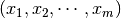$(x_1, x_2, \cdots, x_m)$ . The objective function is

$J = \sum_{i=1}^{m}\sum_{k=1}^{K}w_{ik} ||x_i-c_k||^2$

where $w_{ik}=1$ if $x_i$ is in cluster $k$ ; otherwise $w_{ik}=0$ and $c_k$ is the centroid of $x_i$ ‘s cluster.

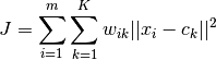
Mathematically, k-means is a minimization problem with two parts: First, we minimize $J$ w.r.t $w_{ik}$ with $c_k$ fixed; Then minimize $J$ w.r.t $c_k$ with $w_{ik}$ fixed. i.e.

E-step:

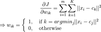
$\frac{\partial J}{\partial w_{ik}} = \sum_{i=1}^{m}\sum_{k=1}^{K} ||x_i-c_k||^2\\ \Rightarrow w_{ik} =\left\{ \begin{array}{ll} 1, & \text{ if }{ k = argmin_{j} ||x_i-c_j||^2} \\ 0, & \text{ otherwise } \end{array} \right.$

M-step:

$\frac{\partial J}{\partial c_k} = 2\sum_{i=1}{m} w_{ik}(x_i-c_k) =0 \Rightarrow c_k = \frac{\sum_{i=1}^{m}w_{ik}x_i}{\sum_{i=1}^{m}w_{ik}}$

12.1.2. Demo¶

Set up spark context and SparkSession

from pyspark.sql import SparkSession

spark = SparkSession \
    .builder \
    .appName("Python Spark K-means example") \
    .config("spark.some.config.option", "some-value") \
    .getOrCreate()

Load dataset

df = spark.read.format('com.databricks.spark.csv').\
                       options(header='true', \
                       inferschema='true').\
            load("../data/iris.csv",header=True);

check the data set

df.show(5,True)
df.printSchema()

Then you will get

+------------+-----------+------------+-----------+-------+
|sepal_length|sepal_width|petal_length|petal_width|species|
+------------+-----------+------------+-----------+-------+
|         5.1|        3.5|         1.4|        0.2| setosa|
|         4.9|        3.0|         1.4|        0.2| setosa|
|         4.7|        3.2|         1.3|        0.2| setosa|
|         4.6|        3.1|         1.5|        0.2| setosa|
|         5.0|        3.6|         1.4|        0.2| setosa|
+------------+-----------+------------+-----------+-------+
only showing top 5 rows

root
 |-- sepal_length: double (nullable = true)
 |-- sepal_width: double (nullable = true)
 |-- petal_length: double (nullable = true)
 |-- petal_width: double (nullable = true)
 |-- species: string (nullable = true)

You can also get the Statistical resutls from the data frame (Unfortunately, it only works for numerical).

df.describe().show()

Then you will get

+-------+------------------+-------------------+------------------+------------------+---------+
|summary|      sepal_length|        sepal_width|      petal_length|       petal_width|  species|
+-------+------------------+-------------------+------------------+------------------+---------+
|  count|               150|                150|               150|               150|      150|
|   mean| 5.843333333333335| 3.0540000000000007|3.7586666666666693|1.1986666666666672|     null|
| stddev|0.8280661279778637|0.43359431136217375| 1.764420419952262|0.7631607417008414|     null|
|    min|               4.3|                2.0|               1.0|               0.1|   setosa|
|    max|               7.9|                4.4|               6.9|               2.5|virginica|
+-------+------------------+-------------------+------------------+------------------+---------+

Convert the data to dense vector (features)

# convert the data to dense vector
from pyspark.mllib.linalg import Vectors
def transData(data):
    return data.rdd.map(lambda r: [Vectors.dense(r[:-1])]).toDF(['features'])

Note

You are strongly encouraged to try my get_dummy function for dealing with the categorical data in complex dataset.

Supervised learning version:

def get_dummy(df,indexCol,categoricalCols,continuousCols,labelCol):

    from pyspark.ml import Pipeline
    from pyspark.ml.feature import StringIndexer, OneHotEncoder, VectorAssembler
    from pyspark.sql.functions import col

    indexers = [ StringIndexer(inputCol=c, outputCol="{0}_indexed".format(c))
                 for c in categoricalCols ]

    # default setting: dropLast=True
    encoders = [ OneHotEncoder(inputCol=indexer.getOutputCol(),
                 outputCol="{0}_encoded".format(indexer.getOutputCol()))
                 for indexer in indexers ]

    assembler = VectorAssembler(inputCols=[encoder.getOutputCol() for encoder in encoders]
                                + continuousCols, outputCol="features")

    pipeline = Pipeline(stages=indexers + encoders + [assembler])

    model=pipeline.fit(df)
    data = model.transform(df)

    data = data.withColumn('label',col(labelCol))

    return data.select(indexCol,'features','label')

Unsupervised learning version:

def get_dummy(df,indexCol,categoricalCols,continuousCols):
    '''
    Get dummy variables and concat with continuous variables for unsupervised learning.
    :param df: the dataframe
    :param categoricalCols: the name list of the categorical data
    :param continuousCols:  the name list of the numerical data
    :return k: feature matrix

    :author: Wenqiang Feng
    :email:  von198@gmail.com
    '''

    indexers = [ StringIndexer(inputCol=c, outputCol="{0}_indexed".format(c))
                 for c in categoricalCols ]

    # default setting: dropLast=True
    encoders = [ OneHotEncoder(inputCol=indexer.getOutputCol(),
                 outputCol="{0}_encoded".format(indexer.getOutputCol()))
                 for indexer in indexers ]

    assembler = VectorAssembler(inputCols=[encoder.getOutputCol() for encoder in encoders]
                                + continuousCols, outputCol="features")

    pipeline = Pipeline(stages=indexers + encoders + [assembler])

    model=pipeline.fit(df)
    data = model.transform(df)

    return data.select(indexCol,'features')

Two in one:

def get_dummy(df,indexCol,categoricalCols,continuousCols,labelCol,dropLast=False):

    '''
    Get dummy variables and concat with continuous variables for ml modeling.
    :param df: the dataframe
    :param categoricalCols: the name list of the categorical data
    :param continuousCols:  the name list of the numerical data
    :param labelCol:  the name of label column
    :param dropLast:  the flag of drop last column
    :return: feature matrix

    :author: Wenqiang Feng
    :email:  von198@gmail.com

    >>> df = spark.createDataFrame([
                  (0, "a"),
                  (1, "b"),
                  (2, "c"),
                  (3, "a"),
                  (4, "a"),
                  (5, "c")
              ], ["id", "category"])

    >>> indexCol = 'id'
    >>> categoricalCols = ['category']
    >>> continuousCols = []
    >>> labelCol = []

    >>> mat = get_dummy(df,indexCol,categoricalCols,continuousCols,labelCol)
    >>> mat.show()

    >>>
        +---+-------------+
        | id|     features|
        +---+-------------+
        |  0|[1.0,0.0,0.0]|
        |  1|[0.0,0.0,1.0]|
        |  2|[0.0,1.0,0.0]|
        |  3|[1.0,0.0,0.0]|
        |  4|[1.0,0.0,0.0]|
        |  5|[0.0,1.0,0.0]|
        +---+-------------+
    '''

    from pyspark.ml import Pipeline
    from pyspark.ml.feature import StringIndexer, OneHotEncoder, VectorAssembler
    from pyspark.sql.functions import col

    indexers = [ StringIndexer(inputCol=c, outputCol="{0}_indexed".format(c))
                 for c in categoricalCols ]

    # default setting: dropLast=True
    encoders = [ OneHotEncoder(inputCol=indexer.getOutputCol(),
                 outputCol="{0}_encoded".format(indexer.getOutputCol()),dropLast=dropLast)
                 for indexer in indexers ]

    assembler = VectorAssembler(inputCols=[encoder.getOutputCol() for encoder in encoders]
                                + continuousCols, outputCol="features")

    pipeline = Pipeline(stages=indexers + encoders + [assembler])

    model=pipeline.fit(df)
    data = model.transform(df)

    if indexCol and labelCol:
        # for supervised learning
        data = data.withColumn('label',col(labelCol))
        return data.select(indexCol,'features','label')
    elif not indexCol and labelCol:
        # for supervised learning
        data = data.withColumn('label',col(labelCol))
        return data.select('features','label')
    elif indexCol and not labelCol:
        # for unsupervised learning
        return data.select(indexCol,'features')
    elif not indexCol and not labelCol:
        # for unsupervised learning
        return data.select('features')

Transform the dataset to DataFrame

transformed= transData(df)
transformed.show(5, False)

+-----------------+
|features         |
+-----------------+
|[5.1,3.5,1.4,0.2]|
|[4.9,3.0,1.4,0.2]|
|[4.7,3.2,1.3,0.2]|
|[4.6,3.1,1.5,0.2]|
|[5.0,3.6,1.4,0.2]|
+-----------------+
only showing top 5 rows

Deal With Categorical Variables

from pyspark.ml import Pipeline
from pyspark.ml.regression import LinearRegression
from pyspark.ml.feature import VectorIndexer
from pyspark.ml.evaluation import RegressionEvaluator

# Automatically identify categorical features, and index them.
# We specify maxCategories so features with > 4 distinct values are treated as continuous.

featureIndexer = VectorIndexer(inputCol="features", \
                               outputCol="indexedFeatures",\
                               maxCategories=4).fit(transformed)

data = featureIndexer.transform(transformed)

Now you check your dataset with

data.show(5,True)

you will get

+-----------------+-----------------+
|         features|  indexedFeatures|
+-----------------+-----------------+
|[5.1,3.5,1.4,0.2]|[5.1,3.5,1.4,0.2]|
|[4.9,3.0,1.4,0.2]|[4.9,3.0,1.4,0.2]|
|[4.7,3.2,1.3,0.2]|[4.7,3.2,1.3,0.2]|
|[4.6,3.1,1.5,0.2]|[4.6,3.1,1.5,0.2]|
|[5.0,3.6,1.4,0.2]|[5.0,3.6,1.4,0.2]|
+-----------------+-----------------+
only showing top 5 rows

Note

Since clustering algorithms including k-means use distance-based measurements to determine the similarity between data points, It’s strongly recommended to standardize the data to have a mean of zero and a standard deviation of one.

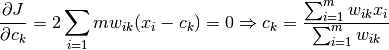
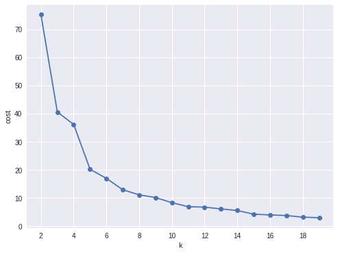
Elbow method to determine the optimal number of clusters for k-means clustering

import numpy as np
cost = np.zeros(20)
for k in range(2,20):
    kmeans = KMeans()\
            .setK(k)\
            .setSeed(1) \
            .setFeaturesCol("indexedFeatures")\
            .setPredictionCol("cluster")

    model = kmeans.fit(data)
    cost[k] = model.computeCost(data) # requires Spark 2.0 or later

import numpy as np
import matplotlib.mlab as mlab
import matplotlib.pyplot as plt
import seaborn as sbs
from matplotlib.ticker import MaxNLocator

fig, ax = plt.subplots(1,1, figsize =(8,6))
ax.plot(range(2,20),cost[2:20])
ax.set_xlabel('k')
ax.set_ylabel('cost')
ax.xaxis.set_major_locator(MaxNLocator(integer=True))
plt.show()

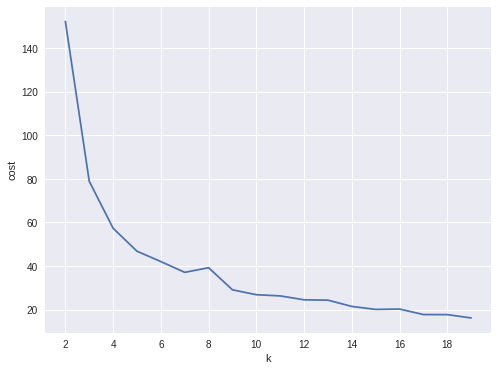
In my opinion, sometimes it’s hard to choose the optimal number of the clusters by using the elbow method. As shown in the following Figure, you can choose 3, 5 or even 8. I will choose 3 in this demo.

Silhouette analysis

#PySpark libraries
from pyspark.ml import Pipeline
from pyspark.ml.feature import StringIndexer, OneHotEncoder, VectorAssembler
from pyspark.sql.functions import col, percent_rank, lit
from pyspark.sql.window import Window
from pyspark.sql import DataFrame, Row
from pyspark.sql.types import StructType
from functools import reduce  # For Python 3.x

from pyspark.ml.clustering import KMeans
from pyspark.ml.evaluation import ClusteringEvaluator

def optimal_k(df_in,index_col,k_min, k_max,num_runs):
    '''
    Determine optimal number of clusters by using Silhoutte Score Analysis.
    :param df_in: the input dataframe
    :param index_col: the name of the index column
    :param k_min: the minmum number of the clusters
    :param k_max: the maxmum number of the clusters
    :param num_runs: the number of runs for each fixed clusters

    :return k: optimal number of the clusters
    :return silh_lst: Silhouette score
    :return r_table: the running results table

    :author: Wenqiang Feng
    :email:  von198@gmail.com
    '''

    start = time.time()
    silh_lst = []
    k_lst = np.arange(k_min, k_max+1)

    r_table = df_in.select(index_col).toPandas()
    r_table = r_table.set_index(index_col)
    centers = pd.DataFrame()

    for k in k_lst:
        silh_val = []
        for run in np.arange(1, num_runs+1):

            # Trains a k-means model.
            kmeans = KMeans()\
                    .setK(k)\
                    .setSeed(int(np.random.randint(100, size=1)))
            model = kmeans.fit(df_in)

            # Make predictions
            predictions = model.transform(df_in)
            r_table['cluster_{k}_{run}'.format(k=k, run=run)]= predictions.select('prediction').toPandas()

            # Evaluate clustering by computing Silhouette score
            evaluator = ClusteringEvaluator()
            silhouette = evaluator.evaluate(predictions)
            silh_val.append(silhouette)

        silh_array=np.asanyarray(silh_val)
        silh_lst.append(silh_array.mean())

    elapsed =  time.time() - start

    silhouette = pd.DataFrame(list(zip(k_lst,silh_lst)),columns = ['k', 'silhouette'])

    print('+------------------------------------------------------------+')
    print("|         The finding optimal k phase took %8.0f s.       |" %(elapsed))
    print('+------------------------------------------------------------+')


    return k_lst[np.argmax(silh_lst, axis=0)], silhouette , r_table

k, silh_lst, r_table = optimal_k(scaledData,index_col,k_min, k_max,num_runs)

+------------------------------------------------------------+
|         The finding optimal k phase took     1783 s.       |
+------------------------------------------------------------+

spark.createDataFrame(silh_lst).show()

+---+------------------+
|  k|        silhouette|
+---+------------------+
|  3|0.8045154385557953|
|  4|0.6993528775512052|
|  5|0.6689286654221447|
|  6|0.6356184024841809|
|  7|0.7174102265711756|
|  8|0.6720861758298997|
|  9| 0.601771359881241|
| 10|0.6292447334578428|
+---+------------------+

From the silhouette list, we can choose 3 as the optimal number of the clusters.

Warning

ClusteringEvaluator in pyspark.ml.evaluation requires Spark 2.4 or later!!

Pipeline Architecture

from pyspark.ml.clustering import KMeans, KMeansModel

kmeans = KMeans() \
          .setK(3) \
          .setFeaturesCol("indexedFeatures")\
          .setPredictionCol("cluster")

# Chain indexer and tree in a Pipeline
pipeline = Pipeline(stages=[featureIndexer, kmeans])

model = pipeline.fit(transformed)

cluster = model.transform(transformed)

k-means clusters

cluster = model.transform(transformed)

+-----------------+-----------------+-------+
|         features|  indexedFeatures|cluster|
+-----------------+-----------------+-------+
|[5.1,3.5,1.4,0.2]|[5.1,3.5,1.4,0.2]|      1|
|[4.9,3.0,1.4,0.2]|[4.9,3.0,1.4,0.2]|      1|
|[4.7,3.2,1.3,0.2]|[4.7,3.2,1.3,0.2]|      1|
|[4.6,3.1,1.5,0.2]|[4.6,3.1,1.5,0.2]|      1|
|[5.0,3.6,1.4,0.2]|[5.0,3.6,1.4,0.2]|      1|
|[5.4,3.9,1.7,0.4]|[5.4,3.9,1.7,0.4]|      1|
|[4.6,3.4,1.4,0.3]|[4.6,3.4,1.4,0.3]|      1|
|[5.0,3.4,1.5,0.2]|[5.0,3.4,1.5,0.2]|      1|
|[4.4,2.9,1.4,0.2]|[4.4,2.9,1.4,0.2]|      1|
|[4.9,3.1,1.5,0.1]|[4.9,3.1,1.5,0.1]|      1|
|[5.4,3.7,1.5,0.2]|[5.4,3.7,1.5,0.2]|      1|
|[4.8,3.4,1.6,0.2]|[4.8,3.4,1.6,0.2]|      1|
|[4.8,3.0,1.4,0.1]|[4.8,3.0,1.4,0.1]|      1|
|[4.3,3.0,1.1,0.1]|[4.3,3.0,1.1,0.1]|      1|
|[5.8,4.0,1.2,0.2]|[5.8,4.0,1.2,0.2]|      1|
|[5.7,4.4,1.5,0.4]|[5.7,4.4,1.5,0.4]|      1|
|[5.4,3.9,1.3,0.4]|[5.4,3.9,1.3,0.4]|      1|
|[5.1,3.5,1.4,0.3]|[5.1,3.5,1.4,0.3]|      1|
|[5.7,3.8,1.7,0.3]|[5.7,3.8,1.7,0.3]|      1|
|[5.1,3.8,1.5,0.3]|[5.1,3.8,1.5,0.3]|      1|
+-----------------+-----------------+-------+
only showing top 20 rows