9. Regression¶

Chinese proverb

A journey of a thousand miles begins with a single step. – old Chinese proverb

In statistical modeling, regression analysis focuses on investigating the relationship between a dependent variable and one or more independent variables. Wikipedia Regression analysis

In data mining, Regression is a model to represent the relationship between the value of lable ( or target, it is numerical variable) and on one or more features (or predictors they can be numerical and categorical variables).

9.1. Linear Regression¶

9.1.1. Introduction¶

Given that a data set $\{\,x_{i1},\ldots ,x_{in},y_{i}\}_{i=1}^{m}$ which contains n features (variables) and m samples (data points), in simple linear regression model for modeling $m$ data points with $j$ independent variables: $x_{ij}$ , the formula is given by:

$y_i = \beta_0 + \beta_j x_{ij}, \text{where}, i= 1, \cdots m, j= 1, \cdots n.$

In matrix notation, the data set is written as $\X = [\x_1,\cdots, \x_n]$ with $\x_j = {\displaystyle \{x_{ij}\}_{i=1}^{m}}$ , $\y = {\displaystyle \{y_{i}\}_{i=1}^{m}}$ (see Fig. Feature matrix and label) and $\Bbeta^\top = {\displaystyle \{\beta_{j}\}_{j=1}^{n}}$ . Then the matrix format equation is written as

(1)¶ $\y = \X \Bbeta.$

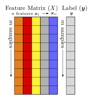
Feature matrix and label¶

9.1.2. How to solve it?¶

Direct Methods (For more information please refer to my Prelim Notes for Numerical Analysis)
- For squared or rectangular matrices
  Singular Value Decomposition
  
  Gram-Schmidt orthogonalization
  
  QR Decomposition
- For squared matrices
  LU Decomposition
  
  Cholesky Decomposition
  
  Regular Splittings
Iterative Methods
- Stationary cases iterative method
  Jacobi Method
  
  Gauss-Seidel Method
  
  Richardson Method
  
  Successive Over Relaxation (SOR) Method
- Dynamic cases iterative method
  Chebyshev iterative Method
  
  Minimal residuals Method
  
  Minimal correction iterative method
  
  Steepest Descent Method
  
  Conjugate Gradients Method

9.1.3. Ordinary Least Squares¶

In mathematics, (1) is a overdetermined system. The method of ordinary least squares can be used to find an approximate solution to overdetermined systems. For the system overdetermined system (1), the least squares formula is obtained from the problem

(2)¶ ${\displaystyle \min _{\Bbeta} ||\X \Bbeta-\y||} ,$

the solution of which can be written with the normal equations:

(3)¶ $\Bbeta = (\X^T\X)^{-1}\X^T\y$

where ${\mathrm {T} }$ indicates a matrix transpose, provided $(\X^{\mathrm {T} }\X)^{-1}$ exists (that is, provided $\X$ has full column rank).

Note

Actually, (3) can be derivated by the following way: multiply $\X^T$ on side of (1) and then multiply $(\X^T\X)^{-1}$ on both side of the former result. You may also apply the Extreme Value Theorem to (2) and find the solution (3).

9.1.4. Gradient Descent¶

Let’s use the following hypothesis:

$h_\Bbeta = \beta_0 + \beta_j \x_{j}, \text{where}, j= 1, \cdots n.$

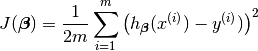
Then, solving (2) is equivalent to minimize the following cost fucntion :

9.1.5. Cost Function¶

(4)¶ $J(\Bbeta) = \frac{1}{2m}\sum_{i=1}^m \left( h_\Bbeta(x^{(i)})-y^{(i)}) \right)^2$

Note

The reason why we prefer to solve (4) rather than (2) is because (4) is convex and it has some nice properties, such as it’s uniquely solvable and energy stable for small enough learning rate. the interested reader who has great interest in non-convex cost function (energy) case. is referred to [Feng2016PSD] for more details.

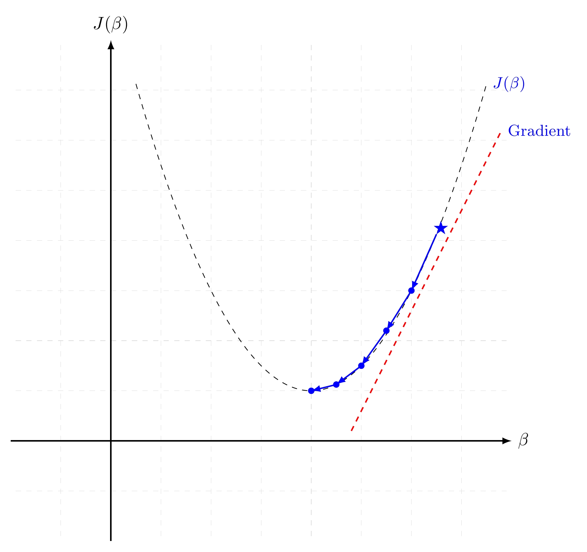
Gradient Descent in 1D¶

Gradient Descent in 2D¶

9.1.6. Batch Gradient Descent¶

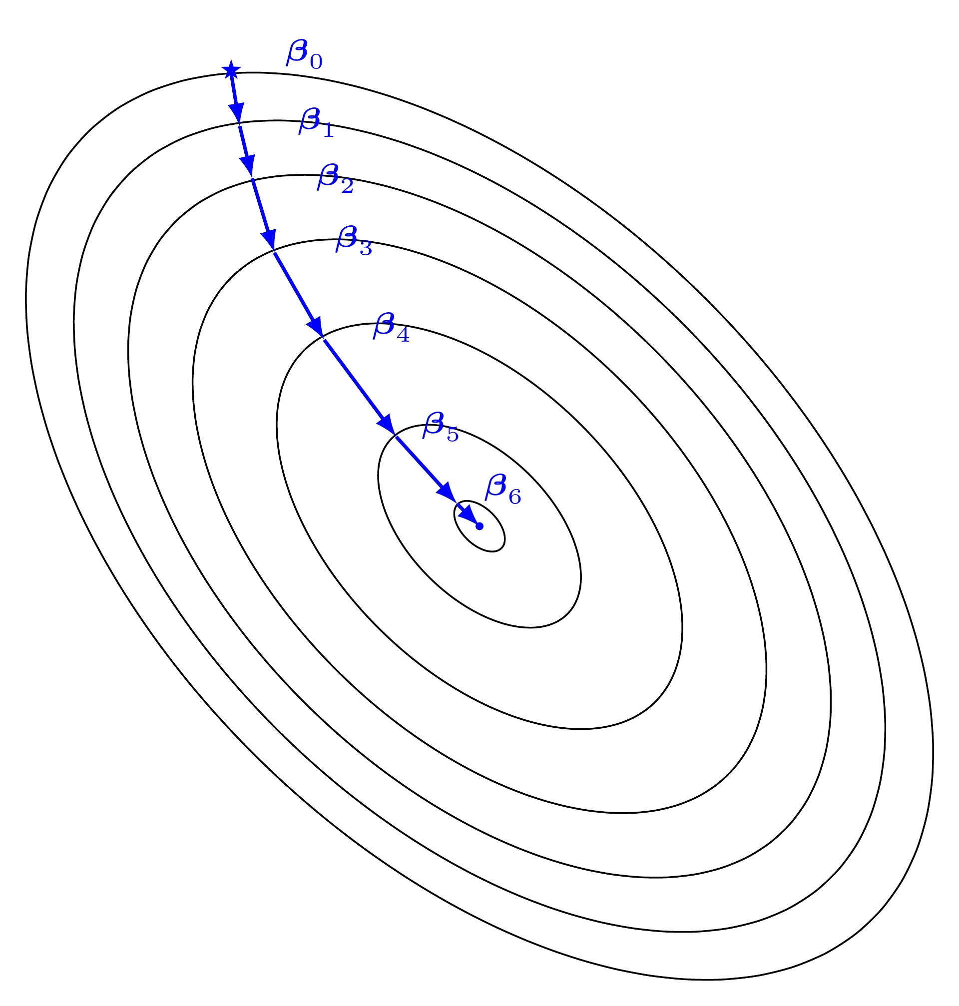
Gradient descent is a first-order iterative optimization algorithm for finding the minimum of a function. It searchs with the direction of the steepest desscent which is defined by the negative of the gradient (see Fig. Gradient Descent in 1D and Gradient Descent in 2D for 1D and 2D, respectively) and with learning rate (search step) $\alpha$ .

9.1.7. Stochastic Dradient Descent¶

9.1.8. Mini-batch Gradient Descent¶

9.1.9. Demo¶

The Jupyter notebook can be download from Linear Regression which was implemented without using Pipeline.
The Jupyter notebook can be download from Linear Regression with Pipeline which was implemented with using Pipeline.
I will only present the code with pipeline style in the following.
For more details about the parameters, please visit Linear Regression API .

Set up spark context and SparkSession

from pyspark.sql import SparkSession

spark = SparkSession \
    .builder \
    .appName("Python Spark regression example") \
    .config("spark.some.config.option", "some-value") \
    .getOrCreate()

Load dataset

df = spark.read.format('com.databricks.spark.csv').\
                       options(header='true', \
                       inferschema='true').\
            load("../data/Advertising.csv",header=True);

check the data set

df.show(5,True)
df.printSchema()

Then you will get

+-----+-----+---------+-----+
|   TV|Radio|Newspaper|Sales|
+-----+-----+---------+-----+
|230.1| 37.8|     69.2| 22.1|
| 44.5| 39.3|     45.1| 10.4|
| 17.2| 45.9|     69.3|  9.3|
|151.5| 41.3|     58.5| 18.5|
|180.8| 10.8|     58.4| 12.9|
+-----+-----+---------+-----+
only showing top 5 rows

root
 |-- TV: double (nullable = true)
 |-- Radio: double (nullable = true)
 |-- Newspaper: double (nullable = true)
 |-- Sales: double (nullable = true)

You can also get the Statistical results from the data frame (Unfortunately, it only works for numerical).

df.describe().show()

Then you will get

+-------+-----------------+------------------+------------------+------------------+
|summary|               TV|             Radio|         Newspaper|             Sales|
+-------+-----------------+------------------+------------------+------------------+
|  count|              200|               200|               200|               200|
|   mean|         147.0425|23.264000000000024|30.553999999999995|14.022500000000003|
| stddev|85.85423631490805|14.846809176168728| 21.77862083852283| 5.217456565710477|
|    min|              0.7|               0.0|               0.3|               1.6|
|    max|            296.4|              49.6|             114.0|              27.0|
+-------+-----------------+------------------+------------------+------------------+

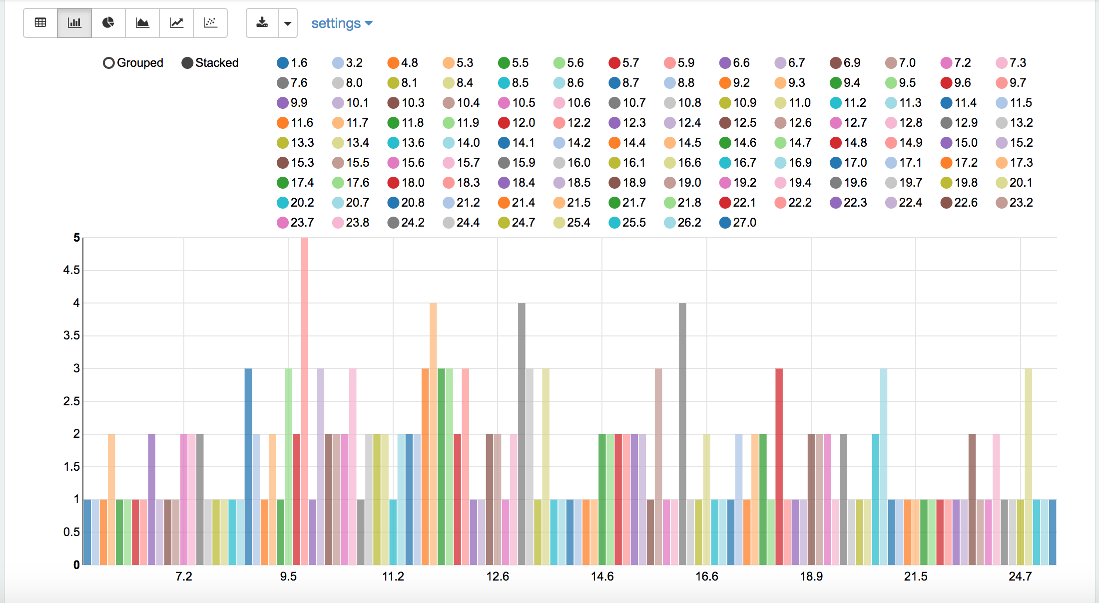
Sales distribution¶

Convert the data to dense vector (features and label)

from pyspark.sql import Row
from pyspark.ml.linalg import Vectors

# I provide two ways to build the features and labels

# method 1 (good for small feature):
#def transData(row):
#    return Row(label=row["Sales"],
#               features=Vectors.dense([row["TV"],
#                                       row["Radio"],
#                                       row["Newspaper"]]))

# Method 2 (good for large features):
def transData(data):
return data.rdd.map(lambda r: [Vectors.dense(r[:-1]),r[-1]]).toDF(['features','label'])

Note

You are strongly encouraged to try my get_dummy function for dealing with the categorical data in comple dataset.

Supervised learning version:

def get_dummy(df,indexCol,categoricalCols,continuousCols,labelCol):

    from pyspark.ml import Pipeline
    from pyspark.ml.feature import StringIndexer, OneHotEncoder, VectorAssembler
    from pyspark.sql.functions import col

    indexers = [ StringIndexer(inputCol=c, outputCol="{0}_indexed".format(c))
                 for c in categoricalCols ]

    # default setting: dropLast=True
    encoders = [ OneHotEncoder(inputCol=indexer.getOutputCol(),
                 outputCol="{0}_encoded".format(indexer.getOutputCol()))
                 for indexer in indexers ]

    assembler = VectorAssembler(inputCols=[encoder.getOutputCol() for encoder in encoders]
                                + continuousCols, outputCol="features")

    pipeline = Pipeline(stages=indexers + encoders + [assembler])

    model=pipeline.fit(df)
    data = model.transform(df)

    data = data.withColumn('label',col(labelCol))

    if indexCol:
        return data.select(indexCol,'features','label')
    else:
        return data.select('features','label')

Unsupervised learning version:

def get_dummy(df,indexCol,categoricalCols,continuousCols):
    '''
    Get dummy variables and concat with continuous variables for unsupervised learning.
    :param df: the dataframe
    :param categoricalCols: the name list of the categorical data
    :param continuousCols:  the name list of the numerical data
    :return k: feature matrix

    :author: Wenqiang Feng
    :email:  von198@gmail.com
    '''

    indexers = [ StringIndexer(inputCol=c, outputCol="{0}_indexed".format(c))
                 for c in categoricalCols ]

    # default setting: dropLast=True
    encoders = [ OneHotEncoder(inputCol=indexer.getOutputCol(),
                 outputCol="{0}_encoded".format(indexer.getOutputCol()))
                 for indexer in indexers ]

    assembler = VectorAssembler(inputCols=[encoder.getOutputCol() for encoder in encoders]
                                + continuousCols, outputCol="features")

    pipeline = Pipeline(stages=indexers + encoders + [assembler])

    model=pipeline.fit(df)
    data = model.transform(df)

    if indexCol:
        return data.select(indexCol,'features')
    else:
        return data.select('features')

Two in one:

def get_dummy(df,indexCol,categoricalCols,continuousCols,labelCol,dropLast=False):

    '''
    Get dummy variables and concat with continuous variables for ml modeling.
    :param df: the dataframe
    :param categoricalCols: the name list of the categorical data
    :param continuousCols:  the name list of the numerical data
    :param labelCol:  the name of label column
    :param dropLast:  the flag of drop last column
    :return: feature matrix

    :author: Wenqiang Feng
    :email:  von198@gmail.com

    >>> df = spark.createDataFrame([
                  (0, "a"),
                  (1, "b"),
                  (2, "c"),
                  (3, "a"),
                  (4, "a"),
                  (5, "c")
              ], ["id", "category"])

    >>> indexCol = 'id'
    >>> categoricalCols = ['category']
    >>> continuousCols = []
    >>> labelCol = []

    >>> mat = get_dummy(df,indexCol,categoricalCols,continuousCols,labelCol)
    >>> mat.show()

    >>>
        +---+-------------+
        | id|     features|
        +---+-------------+
        |  0|[1.0,0.0,0.0]|
        |  1|[0.0,0.0,1.0]|
        |  2|[0.0,1.0,0.0]|
        |  3|[1.0,0.0,0.0]|
        |  4|[1.0,0.0,0.0]|
        |  5|[0.0,1.0,0.0]|
        +---+-------------+
    '''

    from pyspark.ml import Pipeline
    from pyspark.ml.feature import StringIndexer, OneHotEncoder, VectorAssembler
    from pyspark.sql.functions import col

    indexers = [ StringIndexer(inputCol=c, outputCol="{0}_indexed".format(c))
                 for c in categoricalCols ]

    # default setting: dropLast=True
    encoders = [ OneHotEncoder(inputCol=indexer.getOutputCol(),
                 outputCol="{0}_encoded".format(indexer.getOutputCol()),dropLast=dropLast)
                 for indexer in indexers ]

    assembler = VectorAssembler(inputCols=[encoder.getOutputCol() for encoder in encoders]
                                + continuousCols, outputCol="features")

    pipeline = Pipeline(stages=indexers + encoders + [assembler])

    model=pipeline.fit(df)
    data = model.transform(df)

    if indexCol and labelCol:
        # for supervised learning
        data = data.withColumn('label',col(labelCol))
        return data.select(indexCol,'features','label')
    elif not indexCol and labelCol:
        # for supervised learning
        data = data.withColumn('label',col(labelCol))
        return data.select('features','label')
    elif indexCol and not labelCol:
        # for unsupervised learning
        return data.select(indexCol,'features')
    elif not indexCol and not labelCol:
        # for unsupervised learning
        return data.select('features')

Transform the dataset to DataFrame

transformed= transData(df)
transformed.show(5)

+-----------------+-----+
|         features|label|
+-----------------+-----+
|[230.1,37.8,69.2]| 22.1|
| [44.5,39.3,45.1]| 10.4|
| [17.2,45.9,69.3]|  9.3|
|[151.5,41.3,58.5]| 18.5|
|[180.8,10.8,58.4]| 12.9|
+-----------------+-----+
only showing top 5 rows

Note

You will find out that all of the supervised machine learning algorithms in Spark are based on the features and label (unsupervised machine learning algorithms in Spark are based on the features). That is to say, you can play with all of the machine learning algorithms in Spark when you get ready the features and label in pipeline architecture.

Deal With Categorical Variables

from pyspark.ml import Pipeline
from pyspark.ml.regression import LinearRegression
from pyspark.ml.feature import VectorIndexer
from pyspark.ml.evaluation import RegressionEvaluator

# Automatically identify categorical features, and index them.
# We specify maxCategories so features with > 4 distinct values are treated as continuous.

featureIndexer = VectorIndexer(inputCol="features", \
                               outputCol="indexedFeatures",\
                               maxCategories=4).fit(transformed)

data = featureIndexer.transform(transformed)

Now you check your dataset with

data.show(5,True)

you will get

+-----------------+-----+-----------------+
|         features|label|  indexedFeatures|
+-----------------+-----+-----------------+
|[230.1,37.8,69.2]| 22.1|[230.1,37.8,69.2]|
| [44.5,39.3,45.1]| 10.4| [44.5,39.3,45.1]|
| [17.2,45.9,69.3]|  9.3| [17.2,45.9,69.3]|
|[151.5,41.3,58.5]| 18.5|[151.5,41.3,58.5]|
|[180.8,10.8,58.4]| 12.9|[180.8,10.8,58.4]|
+-----------------+-----+-----------------+
only showing top 5 rows

Split the data into training and test sets (40% held out for testing)

# Split the data into training and test sets (40% held out for testing)
(trainingData, testData) = transformed.randomSplit([0.6, 0.4])

You can check your train and test data as follows (In my opinion, it is always to good to keep tracking your data during prototype pahse):

trainingData.show(5)
testData.show(5)

Then you will get

+---------------+-----+---------------+
|       features|label|indexedFeatures|
+---------------+-----+---------------+
| [4.1,11.6,5.7]|  3.2| [4.1,11.6,5.7]|
| [5.4,29.9,9.4]|  5.3| [5.4,29.9,9.4]|
|[7.3,28.1,41.4]|  5.5|[7.3,28.1,41.4]|
|[7.8,38.9,50.6]|  6.6|[7.8,38.9,50.6]|
|  [8.6,2.1,1.0]|  4.8|  [8.6,2.1,1.0]|
+---------------+-----+---------------+
only showing top 5 rows

+----------------+-----+----------------+
|        features|label| indexedFeatures|
+----------------+-----+----------------+
|  [0.7,39.6,8.7]|  1.6|  [0.7,39.6,8.7]|
|  [8.4,27.2,2.1]|  5.7|  [8.4,27.2,2.1]|
|[11.7,36.9,45.2]|  7.3|[11.7,36.9,45.2]|
|[13.2,15.9,49.6]|  5.6|[13.2,15.9,49.6]|
|[16.9,43.7,89.4]|  8.7|[16.9,43.7,89.4]|
+----------------+-----+----------------+
only showing top 5 rows

Fit Ordinary Least Square Regression Model

For more details about the parameters, please visit Linear Regression API .

# Import LinearRegression class
from pyspark.ml.regression import LinearRegression

# Define LinearRegression algorithm
lr = LinearRegression()

Pipeline Architecture

# Chain indexer and tree in a Pipeline
pipeline = Pipeline(stages=[featureIndexer, lr])

model = pipeline.fit(trainingData)

Summary of the Model

Spark has a poor summary function for data and model. I wrote a summary function which has similar format as R output for the linear regression in PySpark.

def modelsummary(model):
    import numpy as np
    print ("Note: the last rows are the information for Intercept")
    print ("##","-------------------------------------------------")
    print ("##","  Estimate   |   Std.Error | t Values  |  P-value")
    coef = np.append(list(model.coefficients),model.intercept)
    Summary=model.summary

    for i in range(len(Summary.pValues)):
        print ("##",'{:10.6f}'.format(coef[i]),\
        '{:10.6f}'.format(Summary.coefficientStandardErrors[i]),\
        '{:8.3f}'.format(Summary.tValues[i]),\
        '{:10.6f}'.format(Summary.pValues[i]))

    print ("##",'---')
    print ("##","Mean squared error: % .6f" \
           % Summary.meanSquaredError, ", RMSE: % .6f" \
           % Summary.rootMeanSquaredError )
    print ("##","Multiple R-squared: %f" % Summary.r2, ", \
            Total iterations: %i"% Summary.totalIterations)

modelsummary(model.stages[-1])

You will get the following summary results:

Note: the last rows are the information for Intercept
('##', '-------------------------------------------------')
('##', '  Estimate   |   Std.Error | t Values  |  P-value')
('##', '  0.044186', '  0.001663', '  26.573', '  0.000000')
('##', '  0.206311', '  0.010846', '  19.022', '  0.000000')
('##', '  0.001963', '  0.007467', '   0.263', '  0.793113')
('##', '  2.596154', '  0.379550', '   6.840', '  0.000000')
('##', '---')
('##', 'Mean squared error:  2.588230', ', RMSE:  1.608798')
('##', 'Multiple R-squared: 0.911869', ',             Total iterations: 1')

Make predictions

# Make predictions.
predictions = model.transform(testData)

# Select example rows to display.
predictions.select("features","label","prediction").show(5)

+----------------+-----+------------------+
|        features|label|        prediction|
+----------------+-----+------------------+
|  [0.7,39.6,8.7]|  1.6| 10.81405928637388|
|  [8.4,27.2,2.1]|  5.7| 8.583086404079918|
|[11.7,36.9,45.2]|  7.3|10.814712818232422|
|[13.2,15.9,49.6]|  5.6| 6.557106943899219|
|[16.9,43.7,89.4]|  8.7|12.534151375058645|
+----------------+-----+------------------+
only showing top 5 rows

Evaluation

from pyspark.ml.evaluation import RegressionEvaluator
# Select (prediction, true label) and compute test error
evaluator = RegressionEvaluator(labelCol="label",
                                predictionCol="prediction",
                                metricName="rmse")

rmse = evaluator.evaluate(predictions)
print("Root Mean Squared Error (RMSE) on test data = %g" % rmse)

The final Root Mean Squared Error (RMSE) is as follows:

Root Mean Squared Error (RMSE) on test data = 1.63114

You can also check the $R^2$ value for the test data:

y_true = predictions.select("label").toPandas()
y_pred = predictions.select("prediction").toPandas()

import sklearn.metrics
r2_score = sklearn.metrics.r2_score(y_true, y_pred)
print('r2_score: {0}'.format(r2_score))

Then you will get

r2_score: 0.854486655585

Warning

You should know most softwares are using different formula to calculate the $R^2$ value when no intercept is included in the model. You can get more information from the disscussion at StackExchange.

9.2. Generalized linear regression¶

9.2.1. Introduction¶

9.2.2. How to solve it?¶

9.2.3. Demo¶

The Jupyter notebook can be download from Generalized Linear Regression.
For more details about the parameters, please visit Generalized Linear Regression API .

Set up spark context and SparkSession

from pyspark.sql import SparkSession

spark = SparkSession \
    .builder \
    .appName("Python Spark regression example") \
    .config("spark.some.config.option", "some-value") \
    .getOrCreate()

Load dataset

df = spark.read.format('com.databricks.spark.csv').\
                       options(header='true', \
                       inferschema='true').\
            load("../data/Advertising.csv",header=True);

check the data set

df.show(5,True)
df.printSchema()

Then you will get

+-----+-----+---------+-----+
|   TV|Radio|Newspaper|Sales|
+-----+-----+---------+-----+
|230.1| 37.8|     69.2| 22.1|
| 44.5| 39.3|     45.1| 10.4|
| 17.2| 45.9|     69.3|  9.3|
|151.5| 41.3|     58.5| 18.5|
|180.8| 10.8|     58.4| 12.9|
+-----+-----+---------+-----+
only showing top 5 rows

root
 |-- TV: double (nullable = true)
 |-- Radio: double (nullable = true)
 |-- Newspaper: double (nullable = true)
 |-- Sales: double (nullable = true)

You can also get the Statistical resutls from the data frame (Unfortunately, it only works for numerical).

df.describe().show()

Then you will get

+-------+-----------------+------------------+------------------+------------------+
|summary|               TV|             Radio|         Newspaper|             Sales|
+-------+-----------------+------------------+------------------+------------------+
|  count|              200|               200|               200|               200|
|   mean|         147.0425|23.264000000000024|30.553999999999995|14.022500000000003|
| stddev|85.85423631490805|14.846809176168728| 21.77862083852283| 5.217456565710477|
|    min|              0.7|               0.0|               0.3|               1.6|
|    max|            296.4|              49.6|             114.0|              27.0|
+-------+-----------------+------------------+------------------+------------------+

Convert the data to dense vector (features and label)

Note

You are strongly encouraged to try my get_dummy function for dealing with the categorical data in comple dataset.

Supervised learning version:

def get_dummy(df,indexCol,categoricalCols,continuousCols,labelCol):

    from pyspark.ml import Pipeline
    from pyspark.ml.feature import StringIndexer, OneHotEncoder, VectorAssembler
    from pyspark.sql.functions import col

    indexers = [ StringIndexer(inputCol=c, outputCol="{0}_indexed".format(c))
                 for c in categoricalCols ]

    # default setting: dropLast=True
    encoders = [ OneHotEncoder(inputCol=indexer.getOutputCol(),
                 outputCol="{0}_encoded".format(indexer.getOutputCol()))
                 for indexer in indexers ]

    assembler = VectorAssembler(inputCols=[encoder.getOutputCol() for encoder in encoders]
                                + continuousCols, outputCol="features")

    pipeline = Pipeline(stages=indexers + encoders + [assembler])

    model=pipeline.fit(df)
    data = model.transform(df)

    data = data.withColumn('label',col(labelCol))

    if indexCol:
        return data.select(indexCol,'features','label')
    else:
        return data.select('features','label')

Unsupervised learning version:

def get_dummy(df,indexCol,categoricalCols,continuousCols):
    '''
    Get dummy variables and concat with continuous variables for unsupervised learning.
    :param df: the dataframe
    :param categoricalCols: the name list of the categorical data
    :param continuousCols:  the name list of the numerical data
    :return k: feature matrix

    :author: Wenqiang Feng
    :email:  von198@gmail.com
    '''

    indexers = [ StringIndexer(inputCol=c, outputCol="{0}_indexed".format(c))
                 for c in categoricalCols ]

    # default setting: dropLast=True
    encoders = [ OneHotEncoder(inputCol=indexer.getOutputCol(),
                 outputCol="{0}_encoded".format(indexer.getOutputCol()))
                 for indexer in indexers ]

    assembler = VectorAssembler(inputCols=[encoder.getOutputCol() for encoder in encoders]
                                + continuousCols, outputCol="features")

    pipeline = Pipeline(stages=indexers + encoders + [assembler])

    model=pipeline.fit(df)
    data = model.transform(df)

    if indexCol:
        return data.select(indexCol,'features')
    else:
        return data.select('features')

Two in one:

def get_dummy(df,indexCol,categoricalCols,continuousCols,labelCol,dropLast=False):

    '''
    Get dummy variables and concat with continuous variables for ml modeling.
    :param df: the dataframe
    :param categoricalCols: the name list of the categorical data
    :param continuousCols:  the name list of the numerical data
    :param labelCol:  the name of label column
    :param dropLast:  the flag of drop last column
    :return: feature matrix

    :author: Wenqiang Feng
    :email:  von198@gmail.com

    >>> df = spark.createDataFrame([
                  (0, "a"),
                  (1, "b"),
                  (2, "c"),
                  (3, "a"),
                  (4, "a"),
                  (5, "c")
              ], ["id", "category"])

    >>> indexCol = 'id'
    >>> categoricalCols = ['category']
    >>> continuousCols = []
    >>> labelCol = []

    >>> mat = get_dummy(df,indexCol,categoricalCols,continuousCols,labelCol)
    >>> mat.show()

    >>>
        +---+-------------+
        | id|     features|
        +---+-------------+
        |  0|[1.0,0.0,0.0]|
        |  1|[0.0,0.0,1.0]|
        |  2|[0.0,1.0,0.0]|
        |  3|[1.0,0.0,0.0]|
        |  4|[1.0,0.0,0.0]|
        |  5|[0.0,1.0,0.0]|
        +---+-------------+
    '''

    from pyspark.ml import Pipeline
    from pyspark.ml.feature import StringIndexer, OneHotEncoder, VectorAssembler
    from pyspark.sql.functions import col

    indexers = [ StringIndexer(inputCol=c, outputCol="{0}_indexed".format(c))
                 for c in categoricalCols ]

    # default setting: dropLast=True
    encoders = [ OneHotEncoder(inputCol=indexer.getOutputCol(),
                 outputCol="{0}_encoded".format(indexer.getOutputCol()),dropLast=dropLast)
                 for indexer in indexers ]

    assembler = VectorAssembler(inputCols=[encoder.getOutputCol() for encoder in encoders]
                                + continuousCols, outputCol="features")

    pipeline = Pipeline(stages=indexers + encoders + [assembler])

    model=pipeline.fit(df)
    data = model.transform(df)

    if indexCol and labelCol:
        # for supervised learning
        data = data.withColumn('label',col(labelCol))
        return data.select(indexCol,'features','label')
    elif not indexCol and labelCol:
        # for supervised learning
        data = data.withColumn('label',col(labelCol))
        return data.select('features','label')
    elif indexCol and not labelCol:
        # for unsupervised learning
        return data.select(indexCol,'features')
    elif not indexCol and not labelCol:
        # for unsupervised learning
        return data.select('features')

from pyspark.sql import Row
from pyspark.ml.linalg import Vectors

# I provide two ways to build the features and labels

# method 1 (good for small feature):
#def transData(row):
#    return Row(label=row["Sales"],
#               features=Vectors.dense([row["TV"],
#                                       row["Radio"],
#                                       row["Newspaper"]]))

# Method 2 (good for large features):
def transData(data):
return data.rdd.map(lambda r: [Vectors.dense(r[:-1]),r[-1]]).toDF(['features','label'])

transformed= transData(df)
transformed.show(5)

+-----------------+-----+
|         features|label|
+-----------------+-----+
|[230.1,37.8,69.2]| 22.1|
| [44.5,39.3,45.1]| 10.4|
| [17.2,45.9,69.3]|  9.3|
|[151.5,41.3,58.5]| 18.5|
|[180.8,10.8,58.4]| 12.9|
+-----------------+-----+
only showing top 5 rows

Note

You will find out that all of the machine learning algorithms in Spark are based on the features and label. That is to say, you can play with all of the machine learning algorithms in Spark when you get ready the features and label.

Convert the data to dense vector

# convert the data to dense vector
def transData(data):
    return data.rdd.map(lambda r: [r[-1], Vectors.dense(r[:-1])]).\
           toDF(['label','features'])

from pyspark.sql import Row
from pyspark.ml.linalg import Vectors

data= transData(df)
data.show()

Deal with the Categorical variables

from pyspark.ml import Pipeline
from pyspark.ml.regression import LinearRegression
from pyspark.ml.feature import VectorIndexer
from pyspark.ml.evaluation import RegressionEvaluator

# Automatically identify categorical features, and index them.
# We specify maxCategories so features with > 4
# distinct values are treated as continuous.

featureIndexer = VectorIndexer(inputCol="features", \
                               outputCol="indexedFeatures",\
                               maxCategories=4).fit(transformed)

data = featureIndexer.transform(transformed)

When you check you data at this point, you will get

+-----------------+-----+-----------------+
|         features|label|  indexedFeatures|
+-----------------+-----+-----------------+
|[230.1,37.8,69.2]| 22.1|[230.1,37.8,69.2]|
| [44.5,39.3,45.1]| 10.4| [44.5,39.3,45.1]|
| [17.2,45.9,69.3]|  9.3| [17.2,45.9,69.3]|
|[151.5,41.3,58.5]| 18.5|[151.5,41.3,58.5]|
|[180.8,10.8,58.4]| 12.9|[180.8,10.8,58.4]|
+-----------------+-----+-----------------+
only showing top 5 rows

Split the data into training and test sets (40% held out for testing)

# Split the data into training and test sets (40% held out for testing)
(trainingData, testData) = transformed.randomSplit([0.6, 0.4])

You can check your train and test data as follows (In my opinion, it is always to good to keep tracking your data during prototype phase):

trainingData.show(5)
testData.show(5)

Then you will get

+----------------+-----+----------------+
|        features|label| indexedFeatures|
+----------------+-----+----------------+
|  [5.4,29.9,9.4]|  5.3|  [5.4,29.9,9.4]|
| [7.8,38.9,50.6]|  6.6| [7.8,38.9,50.6]|
|  [8.4,27.2,2.1]|  5.7|  [8.4,27.2,2.1]|
| [8.7,48.9,75.0]|  7.2| [8.7,48.9,75.0]|
|[11.7,36.9,45.2]|  7.3|[11.7,36.9,45.2]|
+----------------+-----+----------------+
only showing top 5 rows

+---------------+-----+---------------+
|       features|label|indexedFeatures|
+---------------+-----+---------------+
| [0.7,39.6,8.7]|  1.6| [0.7,39.6,8.7]|
| [4.1,11.6,5.7]|  3.2| [4.1,11.6,5.7]|
|[7.3,28.1,41.4]|  5.5|[7.3,28.1,41.4]|
|  [8.6,2.1,1.0]|  4.8|  [8.6,2.1,1.0]|
|[17.2,4.1,31.6]|  5.9|[17.2,4.1,31.6]|
+---------------+-----+---------------+
only showing top 5 rows

Fit Generalized Linear Regression Model

# Import LinearRegression class
from pyspark.ml.regression import GeneralizedLinearRegression

# Define LinearRegression algorithm
glr = GeneralizedLinearRegression(family="gaussian", link="identity",\
                                  maxIter=10, regParam=0.3)

Pipeline Architecture

# Chain indexer and tree in a Pipeline
pipeline = Pipeline(stages=[featureIndexer, glr])

model = pipeline.fit(trainingData)

Summary of the Model

Spark has a poor summary function for data and model. I wrote a summary function which has similar format as R output for the linear regression in PySpark.

def modelsummary(model):
    import numpy as np
    print ("Note: the last rows are the information for Intercept")
    print ("##","-------------------------------------------------")
    print ("##","  Estimate   |   Std.Error | t Values  |  P-value")
    coef = np.append(list(model.coefficients),model.intercept)
    Summary=model.summary

    for i in range(len(Summary.pValues)):
        print ("##",'{:10.6f}'.format(coef[i]),\
        '{:10.6f}'.format(Summary.coefficientStandardErrors[i]),\
        '{:8.3f}'.format(Summary.tValues[i]),\
        '{:10.6f}'.format(Summary.pValues[i]))

    print ("##",'---')
#     print ("##","Mean squared error: % .6f" \
#            % Summary.meanSquaredError, ", RMSE: % .6f" \
#            % Summary.rootMeanSquaredError )
#     print ("##","Multiple R-squared: %f" % Summary.r2, ", \
#             Total iterations: %i"% Summary.totalIterations)

modelsummary(model.stages[-1])

You will get the following summary results:

Note: the last rows are the information for Intercept
('##', '-------------------------------------------------')
('##', '  Estimate   |   Std.Error | t Values  |  P-value')
('##', '  0.042857', '  0.001668', '  25.692', '  0.000000')
('##', '  0.199922', '  0.009881', '  20.232', '  0.000000')
('##', ' -0.001957', '  0.006917', '  -0.283', '  0.777757')
('##', '  3.007515', '  0.406389', '   7.401', '  0.000000')
('##', '---')

Make predictions

# Make predictions.
predictions = model.transform(testData)

# Select example rows to display.
predictions.select("features","label","predictedLabel").show(5)

+---------------+-----+------------------+
|       features|label|        prediction|
+---------------+-----+------------------+
| [0.7,39.6,8.7]|  1.6|10.937383732327625|
| [4.1,11.6,5.7]|  3.2| 5.491166258750164|
|[7.3,28.1,41.4]|  5.5|   8.8571603947873|
|  [8.6,2.1,1.0]|  4.8| 3.793966281660073|
|[17.2,4.1,31.6]|  5.9| 4.502507124763654|
+---------------+-----+------------------+
only showing top 5 rows

Evaluation

from pyspark.ml.evaluation import RegressionEvaluator
from pyspark.ml.evaluation import RegressionEvaluator
# Select (prediction, true label) and compute test error
evaluator = RegressionEvaluator(labelCol="label",
                                predictionCol="prediction",
                                metricName="rmse")

rmse = evaluator.evaluate(predictions)
print("Root Mean Squared Error (RMSE) on test data = %g" % rmse)

The final Root Mean Squared Error (RMSE) is as follows:

Root Mean Squared Error (RMSE) on test data = 1.89857

y_true = predictions.select("label").toPandas()
y_pred = predictions.select("prediction").toPandas()

import sklearn.metrics
r2_score = sklearn.metrics.r2_score(y_true, y_pred)
print('r2_score: {0}'.format(r2_score))

Then you will get the $R^2$ value:

r2_score: 0.87707391843

9.3. Decision tree Regression¶

9.3.1. Introduction¶

9.3.2. How to solve it?¶

9.3.3. Demo¶

The Jupyter notebook can be download from Decision Tree Regression.
For more details about the parameters, please visit Decision Tree Regressor API .

Set up spark context and SparkSession

from pyspark.sql import SparkSession

spark = SparkSession \
    .builder \
    .appName("Python Spark regression example") \
    .config("spark.some.config.option", "some-value") \
    .getOrCreate()

Load dataset

df = spark.read.format('com.databricks.spark.csv').\
                       options(header='true', \
                       inferschema='true').\
            load("../data/Advertising.csv",header=True);

check the data set

df.show(5,True)
df.printSchema()

Then you will get

+-----+-----+---------+-----+
|   TV|Radio|Newspaper|Sales|
+-----+-----+---------+-----+
|230.1| 37.8|     69.2| 22.1|
| 44.5| 39.3|     45.1| 10.4|
| 17.2| 45.9|     69.3|  9.3|
|151.5| 41.3|     58.5| 18.5|
|180.8| 10.8|     58.4| 12.9|
+-----+-----+---------+-----+
only showing top 5 rows

root
 |-- TV: double (nullable = true)
 |-- Radio: double (nullable = true)
 |-- Newspaper: double (nullable = true)
 |-- Sales: double (nullable = true)

You can also get the Statistical resutls from the data frame (Unfortunately, it only works for numerical).

df.describe().show()

Then you will get

+-------+-----------------+------------------+------------------+------------------+
|summary|               TV|             Radio|         Newspaper|             Sales|
+-------+-----------------+------------------+------------------+------------------+
|  count|              200|               200|               200|               200|
|   mean|         147.0425|23.264000000000024|30.553999999999995|14.022500000000003|
| stddev|85.85423631490805|14.846809176168728| 21.77862083852283| 5.217456565710477|
|    min|              0.7|               0.0|               0.3|               1.6|
|    max|            296.4|              49.6|             114.0|              27.0|
+-------+-----------------+------------------+------------------+------------------+

Convert the data to dense vector (features and label)

Note

You are strongly encouraged to try my get_dummy function for dealing with the categorical data in comple dataset.

Supervised learning version:

def get_dummy(df,indexCol,categoricalCols,continuousCols,labelCol):

    from pyspark.ml import Pipeline
    from pyspark.ml.feature import StringIndexer, OneHotEncoder, VectorAssembler
    from pyspark.sql.functions import col

    indexers = [ StringIndexer(inputCol=c, outputCol="{0}_indexed".format(c))
                 for c in categoricalCols ]

    # default setting: dropLast=True
    encoders = [ OneHotEncoder(inputCol=indexer.getOutputCol(),
                 outputCol="{0}_encoded".format(indexer.getOutputCol()))
                 for indexer in indexers ]

    assembler = VectorAssembler(inputCols=[encoder.getOutputCol() for encoder in encoders]
                                + continuousCols, outputCol="features")

    pipeline = Pipeline(stages=indexers + encoders + [assembler])

    model=pipeline.fit(df)
    data = model.transform(df)

    data = data.withColumn('label',col(labelCol))

    return data.select(indexCol,'features','label')

Unsupervised learning version:

def get_dummy(df,indexCol,categoricalCols,continuousCols):
    '''
    Get dummy variables and concat with continuous variables for unsupervised learning.
    :param df: the dataframe
    :param categoricalCols: the name list of the categorical data
    :param continuousCols:  the name list of the numerical data
    :return k: feature matrix

    :author: Wenqiang Feng
    :email:  von198@gmail.com
    '''

    indexers = [ StringIndexer(inputCol=c, outputCol="{0}_indexed".format(c))
                 for c in categoricalCols ]

    # default setting: dropLast=True
    encoders = [ OneHotEncoder(inputCol=indexer.getOutputCol(),
                 outputCol="{0}_encoded".format(indexer.getOutputCol()))
                 for indexer in indexers ]

    assembler = VectorAssembler(inputCols=[encoder.getOutputCol() for encoder in encoders]
                                + continuousCols, outputCol="features")

    pipeline = Pipeline(stages=indexers + encoders + [assembler])

    model=pipeline.fit(df)
    data = model.transform(df)

    return data.select(indexCol,'features')

Two in one:

def get_dummy(df,indexCol,categoricalCols,continuousCols,labelCol,dropLast=False):

    '''
    Get dummy variables and concat with continuous variables for ml modeling.
    :param df: the dataframe
    :param categoricalCols: the name list of the categorical data
    :param continuousCols:  the name list of the numerical data
    :param labelCol:  the name of label column
    :param dropLast:  the flag of drop last column
    :return: feature matrix

    :author: Wenqiang Feng
    :email:  von198@gmail.com

    >>> df = spark.createDataFrame([
                  (0, "a"),
                  (1, "b"),
                  (2, "c"),
                  (3, "a"),
                  (4, "a"),
                  (5, "c")
              ], ["id", "category"])

    >>> indexCol = 'id'
    >>> categoricalCols = ['category']
    >>> continuousCols = []
    >>> labelCol = []

    >>> mat = get_dummy(df,indexCol,categoricalCols,continuousCols,labelCol)
    >>> mat.show()

    >>>
        +---+-------------+
        | id|     features|
        +---+-------------+
        |  0|[1.0,0.0,0.0]|
        |  1|[0.0,0.0,1.0]|
        |  2|[0.0,1.0,0.0]|
        |  3|[1.0,0.0,0.0]|
        |  4|[1.0,0.0,0.0]|
        |  5|[0.0,1.0,0.0]|
        +---+-------------+
    '''

    from pyspark.ml import Pipeline
    from pyspark.ml.feature import StringIndexer, OneHotEncoder, VectorAssembler
    from pyspark.sql.functions import col

    indexers = [ StringIndexer(inputCol=c, outputCol="{0}_indexed".format(c))
                 for c in categoricalCols ]

    # default setting: dropLast=True
    encoders = [ OneHotEncoder(inputCol=indexer.getOutputCol(),
                 outputCol="{0}_encoded".format(indexer.getOutputCol()),dropLast=dropLast)
                 for indexer in indexers ]

    assembler = VectorAssembler(inputCols=[encoder.getOutputCol() for encoder in encoders]
                                + continuousCols, outputCol="features")

    pipeline = Pipeline(stages=indexers + encoders + [assembler])

    model=pipeline.fit(df)
    data = model.transform(df)

    if indexCol and labelCol:
        # for supervised learning
        data = data.withColumn('label',col(labelCol))
        return data.select(indexCol,'features','label')
    elif not indexCol and labelCol:
        # for supervised learning
        data = data.withColumn('label',col(labelCol))
        return data.select('features','label')
    elif indexCol and not labelCol:
        # for unsupervised learning
        return data.select(indexCol,'features')
    elif not indexCol and not labelCol:
        # for unsupervised learning
        return data.select('features')

from pyspark.sql import Row
from pyspark.ml.linalg import Vectors

# I provide two ways to build the features and labels

# method 1 (good for small feature):
#def transData(row):
#    return Row(label=row["Sales"],
#               features=Vectors.dense([row["TV"],
#                                       row["Radio"],
#                                       row["Newspaper"]]))

# Method 2 (good for large features):
def transData(data):
return data.rdd.map(lambda r: [Vectors.dense(r[:-1]),r[-1]]).toDF(['features','label'])

transformed= transData(df)
transformed.show(5)

+-----------------+-----+
|         features|label|
+-----------------+-----+
|[230.1,37.8,69.2]| 22.1|
| [44.5,39.3,45.1]| 10.4|
| [17.2,45.9,69.3]|  9.3|
|[151.5,41.3,58.5]| 18.5|
|[180.8,10.8,58.4]| 12.9|
+-----------------+-----+
only showing top 5 rows

Note

You will find out that all of the machine learning algorithms in Spark are based on the features and label. That is to say, you can play with all of the machine learning algorithms in Spark when you get ready the features and label.

Convert the data to dense vector

# convert the data to dense vector
def transData(data):
    return data.rdd.map(lambda r: [r[-1], Vectors.dense(r[:-1])]).\
           toDF(['label','features'])

transformed = transData(df)
transformed.show(5)

Deal with the Categorical variables

from pyspark.ml import Pipeline
from pyspark.ml.regression import LinearRegression
from pyspark.ml.feature import VectorIndexer
from pyspark.ml.evaluation import RegressionEvaluator

# Automatically identify categorical features, and index them.
# We specify maxCategories so features with > 4
# distinct values are treated as continuous.

featureIndexer = VectorIndexer(inputCol="features", \
                               outputCol="indexedFeatures",\
                               maxCategories=4).fit(transformed)

data = featureIndexer.transform(transformed)

When you check you data at this point, you will get

+-----------------+-----+-----------------+
|         features|label|  indexedFeatures|
+-----------------+-----+-----------------+
|[230.1,37.8,69.2]| 22.1|[230.1,37.8,69.2]|
| [44.5,39.3,45.1]| 10.4| [44.5,39.3,45.1]|
| [17.2,45.9,69.3]|  9.3| [17.2,45.9,69.3]|
|[151.5,41.3,58.5]| 18.5|[151.5,41.3,58.5]|
|[180.8,10.8,58.4]| 12.9|[180.8,10.8,58.4]|
+-----------------+-----+-----------------+
only showing top 5 rows

Split the data into training and test sets (40% held out for testing)

# Split the data into training and test sets (40% held out for testing)
(trainingData, testData) = transformed.randomSplit([0.6, 0.4])

You can check your train and test data as follows (In my opinion, it is always to good to keep tracking your data during prototype pahse):

trainingData.show(5)
testData.show(5)

Then you will get

+---------------+-----+---------------+
|       features|label|indexedFeatures|
+---------------+-----+---------------+
| [4.1,11.6,5.7]|  3.2| [4.1,11.6,5.7]|
|[7.3,28.1,41.4]|  5.5|[7.3,28.1,41.4]|
| [8.4,27.2,2.1]|  5.7| [8.4,27.2,2.1]|
|  [8.6,2.1,1.0]|  4.8|  [8.6,2.1,1.0]|
|[8.7,48.9,75.0]|  7.2|[8.7,48.9,75.0]|
+---------------+-----+---------------+
only showing top 5 rows

+----------------+-----+----------------+
|        features|label| indexedFeatures|
+----------------+-----+----------------+
|  [0.7,39.6,8.7]|  1.6|  [0.7,39.6,8.7]|
|  [5.4,29.9,9.4]|  5.3|  [5.4,29.9,9.4]|
| [7.8,38.9,50.6]|  6.6| [7.8,38.9,50.6]|
|[17.2,45.9,69.3]|  9.3|[17.2,45.9,69.3]|
|[18.7,12.1,23.4]|  6.7|[18.7,12.1,23.4]|
+----------------+-----+----------------+
only showing top 5 rows

Fit Decision Tree Regression Model

from pyspark.ml.regression import DecisionTreeRegressor

# Train a DecisionTree model.
dt = DecisionTreeRegressor(featuresCol="indexedFeatures")

Pipeline Architecture

# Chain indexer and tree in a Pipeline
pipeline = Pipeline(stages=[featureIndexer, dt])

model = pipeline.fit(trainingData)

Make predictions

# Make predictions.
predictions = model.transform(testData)

# Select example rows to display.
predictions.select("features","label","predictedLabel").show(5)

+----------+-----+----------------+
|prediction|label|        features|
+----------+-----+----------------+
|       7.2|  1.6|  [0.7,39.6,8.7]|
|       7.3|  5.3|  [5.4,29.9,9.4]|
|       7.2|  6.6| [7.8,38.9,50.6]|
|      8.64|  9.3|[17.2,45.9,69.3]|
|      6.45|  6.7|[18.7,12.1,23.4]|
+----------+-----+----------------+
only showing top 5 rows

Evaluation

from pyspark.ml.evaluation import RegressionEvaluator
from pyspark.ml.evaluation import RegressionEvaluator
# Select (prediction, true label) and compute test error
evaluator = RegressionEvaluator(labelCol="label",
                                predictionCol="prediction",
                                metricName="rmse")

rmse = evaluator.evaluate(predictions)
print("Root Mean Squared Error (RMSE) on test data = %g" % rmse)

The final Root Mean Squared Error (RMSE) is as follows:

Root Mean Squared Error (RMSE) on test data = 1.50999

y_true = predictions.select("label").toPandas()
y_pred = predictions.select("prediction").toPandas()

import sklearn.metrics
r2_score = sklearn.metrics.r2_score(y_true, y_pred)
print('r2_score: {0}'.format(r2_score))

Then you will get the $R^2$ value:

r2_score: 0.911024318967

You may also check the importance of the features:

model.stages[1].featureImportances

The you will get the weight for each features

SparseVector(3, {0: 0.6811, 1: 0.3187, 2: 0.0002})

9.4. Random Forest Regression¶

9.4.1. Introduction¶

9.4.2. How to solve it?¶

9.4.3. Demo¶

The Jupyter notebook can be download from Random Forest Regression.
For more details about the parameters, please visit Random Forest Regressor API .

Set up spark context and SparkSession

from pyspark.sql import SparkSession

spark = SparkSession \
    .builder \
    .appName("Python Spark RandomForest Regression example") \
    .config("spark.some.config.option", "some-value") \
    .getOrCreate()

Load dataset

df = spark.read.format('com.databricks.spark.csv').\
                               options(header='true', \
                               inferschema='true').\
                               load("../data/Advertising.csv",header=True);

df.show(5,True)
df.printSchema()

+-----+-----+---------+-----+
|   TV|Radio|Newspaper|Sales|
+-----+-----+---------+-----+
|230.1| 37.8|     69.2| 22.1|
| 44.5| 39.3|     45.1| 10.4|
| 17.2| 45.9|     69.3|  9.3|
|151.5| 41.3|     58.5| 18.5|
|180.8| 10.8|     58.4| 12.9|
+-----+-----+---------+-----+
only showing top 5 rows

root
 |-- TV: double (nullable = true)
 |-- Radio: double (nullable = true)
 |-- Newspaper: double (nullable = true)
 |-- Sales: double (nullable = true)

df.describe().show()

+-------+-----------------+------------------+------------------+------------------+
|summary|               TV|             Radio|         Newspaper|             Sales|
+-------+-----------------+------------------+------------------+------------------+
|  count|              200|               200|               200|               200|
|   mean|         147.0425|23.264000000000024|30.553999999999995|14.022500000000003|
| stddev|85.85423631490805|14.846809176168728| 21.77862083852283| 5.217456565710477|
|    min|              0.7|               0.0|               0.3|               1.6|
|    max|            296.4|              49.6|             114.0|              27.0|
+-------+-----------------+------------------+------------------+------------------+

Convert the data to dense vector (features and label)

Note

You are strongly encouraged to try my get_dummy function for dealing with the categorical data in comple dataset.

Supervised learning version:

def get_dummy(df,indexCol,categoricalCols,continuousCols,labelCol):

    from pyspark.ml import Pipeline
    from pyspark.ml.feature import StringIndexer, OneHotEncoder, VectorAssembler
    from pyspark.sql.functions import col

    indexers = [ StringIndexer(inputCol=c, outputCol="{0}_indexed".format(c))
                 for c in categoricalCols ]

    # default setting: dropLast=True
    encoders = [ OneHotEncoder(inputCol=indexer.getOutputCol(),
                 outputCol="{0}_encoded".format(indexer.getOutputCol()))
                 for indexer in indexers ]

    assembler = VectorAssembler(inputCols=[encoder.getOutputCol() for encoder in encoders]
                                + continuousCols, outputCol="features")

    pipeline = Pipeline(stages=indexers + encoders + [assembler])

    model=pipeline.fit(df)
    data = model.transform(df)

    data = data.withColumn('label',col(labelCol))

    return data.select(indexCol,'features','label')

Unsupervised learning version:

def get_dummy(df,indexCol,categoricalCols,continuousCols):
    '''
    Get dummy variables and concat with continuous variables for unsupervised learning.
    :param df: the dataframe
    :param categoricalCols: the name list of the categorical data
    :param continuousCols:  the name list of the numerical data
    :return k: feature matrix

    :author: Wenqiang Feng
    :email:  von198@gmail.com
    '''

    indexers = [ StringIndexer(inputCol=c, outputCol="{0}_indexed".format(c))
                 for c in categoricalCols ]

    # default setting: dropLast=True
    encoders = [ OneHotEncoder(inputCol=indexer.getOutputCol(),
                 outputCol="{0}_encoded".format(indexer.getOutputCol()))
                 for indexer in indexers ]

    assembler = VectorAssembler(inputCols=[encoder.getOutputCol() for encoder in encoders]
                                + continuousCols, outputCol="features")

    pipeline = Pipeline(stages=indexers + encoders + [assembler])

    model=pipeline.fit(df)
    data = model.transform(df)

    return data.select(indexCol,'features')

Two in one:

def get_dummy(df,indexCol,categoricalCols,continuousCols,labelCol,dropLast=False):

    '''
    Get dummy variables and concat with continuous variables for ml modeling.
    :param df: the dataframe
    :param categoricalCols: the name list of the categorical data
    :param continuousCols:  the name list of the numerical data
    :param labelCol:  the name of label column
    :param dropLast:  the flag of drop last column
    :return: feature matrix

    :author: Wenqiang Feng
    :email:  von198@gmail.com

    >>> df = spark.createDataFrame([
                  (0, "a"),
                  (1, "b"),
                  (2, "c"),
                  (3, "a"),
                  (4, "a"),
                  (5, "c")
              ], ["id", "category"])

    >>> indexCol = 'id'
    >>> categoricalCols = ['category']
    >>> continuousCols = []
    >>> labelCol = []

    >>> mat = get_dummy(df,indexCol,categoricalCols,continuousCols,labelCol)
    >>> mat.show()

    >>>
        +---+-------------+
        | id|     features|
        +---+-------------+
        |  0|[1.0,0.0,0.0]|
        |  1|[0.0,0.0,1.0]|
        |  2|[0.0,1.0,0.0]|
        |  3|[1.0,0.0,0.0]|
        |  4|[1.0,0.0,0.0]|
        |  5|[0.0,1.0,0.0]|
        +---+-------------+
    '''

    from pyspark.ml import Pipeline
    from pyspark.ml.feature import StringIndexer, OneHotEncoder, VectorAssembler
    from pyspark.sql.functions import col

    indexers = [ StringIndexer(inputCol=c, outputCol="{0}_indexed".format(c))
                 for c in categoricalCols ]

    # default setting: dropLast=True
    encoders = [ OneHotEncoder(inputCol=indexer.getOutputCol(),
                 outputCol="{0}_encoded".format(indexer.getOutputCol()),dropLast=dropLast)
                 for indexer in indexers ]

    assembler = VectorAssembler(inputCols=[encoder.getOutputCol() for encoder in encoders]
                                + continuousCols, outputCol="features")

    pipeline = Pipeline(stages=indexers + encoders + [assembler])

    model=pipeline.fit(df)
    data = model.transform(df)

    if indexCol and labelCol:
        # for supervised learning
        data = data.withColumn('label',col(labelCol))
        return data.select(indexCol,'features','label')
    elif not indexCol and labelCol:
        # for supervised learning
        data = data.withColumn('label',col(labelCol))
        return data.select('features','label')
    elif indexCol and not labelCol:
        # for unsupervised learning
        return data.select(indexCol,'features')
    elif not indexCol and not labelCol:
        # for unsupervised learning
        return data.select('features')

from pyspark.sql import Row
from pyspark.ml.linalg import Vectors

# convert the data to dense vector
#def transData(row):
#    return Row(label=row["Sales"],
#               features=Vectors.dense([row["TV"],
#                                       row["Radio"],
#                                       row["Newspaper"]]))
def transData(data):
    return data.rdd.map(lambda r: [Vectors.dense(r[:-1]),r[-1]]).toDF(['features','label'])

Convert the data to dense vector

transformed= transData(df)
transformed.show(5)

+-----------------+-----+
|         features|label|
+-----------------+-----+
|[230.1,37.8,69.2]| 22.1|
| [44.5,39.3,45.1]| 10.4|
| [17.2,45.9,69.3]|  9.3|
|[151.5,41.3,58.5]| 18.5|
|[180.8,10.8,58.4]| 12.9|
+-----------------+-----+
only showing top 5 rows

Deal with the Categorical variables

from pyspark.ml import Pipeline
from pyspark.ml.regression import LinearRegression
from pyspark.ml.feature import VectorIndexer
from pyspark.ml.evaluation import RegressionEvaluator

featureIndexer = VectorIndexer(inputCol="features", \
                               outputCol="indexedFeatures",\
                               maxCategories=4).fit(transformed)

data = featureIndexer.transform(transformed)
data.show(5,True)

+-----------------+-----+-----------------+
|         features|label|  indexedFeatures|
+-----------------+-----+-----------------+
|[230.1,37.8,69.2]| 22.1|[230.1,37.8,69.2]|
| [44.5,39.3,45.1]| 10.4| [44.5,39.3,45.1]|
| [17.2,45.9,69.3]|  9.3| [17.2,45.9,69.3]|
|[151.5,41.3,58.5]| 18.5|[151.5,41.3,58.5]|
|[180.8,10.8,58.4]| 12.9|[180.8,10.8,58.4]|
+-----------------+-----+-----------------+
only showing top 5 rows

Split the data into training and test sets (40% held out for testing)

# Split the data into training and test sets (40% held out for testing)
(trainingData, testData) = data.randomSplit([0.6, 0.4])

trainingData.show(5)
testData.show(5)

+----------------+-----+----------------+
|        features|label| indexedFeatures|
+----------------+-----+----------------+
|  [0.7,39.6,8.7]|  1.6|  [0.7,39.6,8.7]|
|   [8.6,2.1,1.0]|  4.8|   [8.6,2.1,1.0]|
| [8.7,48.9,75.0]|  7.2| [8.7,48.9,75.0]|
|[11.7,36.9,45.2]|  7.3|[11.7,36.9,45.2]|
|[13.2,15.9,49.6]|  5.6|[13.2,15.9,49.6]|
+----------------+-----+----------------+
only showing top 5 rows

+---------------+-----+---------------+
|       features|label|indexedFeatures|
+---------------+-----+---------------+
| [4.1,11.6,5.7]|  3.2| [4.1,11.6,5.7]|
| [5.4,29.9,9.4]|  5.3| [5.4,29.9,9.4]|
|[7.3,28.1,41.4]|  5.5|[7.3,28.1,41.4]|
|[7.8,38.9,50.6]|  6.6|[7.8,38.9,50.6]|
| [8.4,27.2,2.1]|  5.7| [8.4,27.2,2.1]|
+---------------+-----+---------------+
only showing top 5 rows

Fit RandomForest Regression Model

# Import LinearRegression class
from pyspark.ml.regression import RandomForestRegressor

# Define LinearRegression algorithm
rf = RandomForestRegressor() # featuresCol="indexedFeatures",numTrees=2, maxDepth=2, seed=42

Note

If you decide to use the indexedFeatures features, you need to add the parameter featuresCol="indexedFeatures".

Pipeline Architecture

# Chain indexer and tree in a Pipeline
pipeline = Pipeline(stages=[featureIndexer, rf])
model = pipeline.fit(trainingData)

Make predictions

predictions = model.transform(testData)

# Select example rows to display.
predictions.select("features","label", "prediction").show(5)

+---------------+-----+------------------+
|       features|label|        prediction|
+---------------+-----+------------------+
| [4.1,11.6,5.7]|  3.2| 8.155439814814816|
| [5.4,29.9,9.4]|  5.3|10.412769901394899|
|[7.3,28.1,41.4]|  5.5| 12.13735648148148|
|[7.8,38.9,50.6]|  6.6|11.321796703296704|
| [8.4,27.2,2.1]|  5.7|12.071421957671957|
+---------------+-----+------------------+
only showing top 5 rows

Evaluation

# Select (prediction, true label) and compute test error
evaluator = RegressionEvaluator(
    labelCol="label", predictionCol="prediction", metricName="rmse")
rmse = evaluator.evaluate(predictions)
print("Root Mean Squared Error (RMSE) on test data = %g" % rmse)

Root Mean Squared Error (RMSE) on test data = 2.35912

import sklearn.metrics
r2_score = sklearn.metrics.r2_score(y_true, y_pred)
print('r2_score: {:4.3f}'.format(r2_score))

r2_score: 0.831

Feature importances

model.stages[-1].featureImportances

SparseVector(3, {0: 0.4994, 1: 0.3196, 2: 0.181})

model.stages[-1].trees

[DecisionTreeRegressionModel (uid=dtr_c75f1c75442c) of depth 5 with 43 nodes,
 DecisionTreeRegressionModel (uid=dtr_70fc2d441581) of depth 5 with 45 nodes,
 DecisionTreeRegressionModel (uid=dtr_bc8464f545a7) of depth 5 with 31 nodes,
 DecisionTreeRegressionModel (uid=dtr_a8a7e5367154) of depth 5 with 59 nodes,
 DecisionTreeRegressionModel (uid=dtr_3ea01314fcbc) of depth 5 with 47 nodes,
 DecisionTreeRegressionModel (uid=dtr_be9a04ac22a6) of depth 5 with 45 nodes,
 DecisionTreeRegressionModel (uid=dtr_38610d47328a) of depth 5 with 51 nodes,
 DecisionTreeRegressionModel (uid=dtr_bf14aea0ad3b) of depth 5 with 49 nodes,
 DecisionTreeRegressionModel (uid=dtr_cde24ebd6bb6) of depth 5 with 39 nodes,
 DecisionTreeRegressionModel (uid=dtr_a1fc9bd4fbeb) of depth 5 with 57 nodes,
 DecisionTreeRegressionModel (uid=dtr_37798d6db1ba) of depth 5 with 41 nodes,
 DecisionTreeRegressionModel (uid=dtr_c078b73ada63) of depth 5 with 41 nodes,
 DecisionTreeRegressionModel (uid=dtr_fd00e3a070ad) of depth 5 with 55 nodes,
 DecisionTreeRegressionModel (uid=dtr_9d01d5fb8604) of depth 5 with 45 nodes,
 DecisionTreeRegressionModel (uid=dtr_8bd8bdddf642) of depth 5 with 41 nodes,
 DecisionTreeRegressionModel (uid=dtr_e53b7bae30f8) of depth 5 with 49 nodes,
 DecisionTreeRegressionModel (uid=dtr_808a869db21c) of depth 5 with 47 nodes,
 DecisionTreeRegressionModel (uid=dtr_64d0916bceb0) of depth 5 with 33 nodes,
 DecisionTreeRegressionModel (uid=dtr_0891055fff94) of depth 5 with 55 nodes,
 DecisionTreeRegressionModel (uid=dtr_19c8bbad26c2) of depth 5 with 51 nodes]

9.5. Gradient-boosted tree regression¶

9.5.1. Introduction¶

9.5.2. How to solve it?¶

9.5.3. Demo¶

The Jupyter notebook can be download from Gradient-boosted tree regression.
For more details about the parameters, please visit Gradient boosted tree API .

Set up spark context and SparkSession

from pyspark.sql import SparkSession

spark = SparkSession \
    .builder \
    .appName("Python Spark GBTRegressor example") \
    .config("spark.some.config.option", "some-value") \
    .getOrCreate()

Load dataset

df = spark.read.format('com.databricks.spark.csv').\
                               options(header='true', \
                               inferschema='true').\
                               load("../data/Advertising.csv",header=True);

df.show(5,True)
df.printSchema()

+-----+-----+---------+-----+
|   TV|Radio|Newspaper|Sales|
+-----+-----+---------+-----+
|230.1| 37.8|     69.2| 22.1|
| 44.5| 39.3|     45.1| 10.4|
| 17.2| 45.9|     69.3|  9.3|
|151.5| 41.3|     58.5| 18.5|
|180.8| 10.8|     58.4| 12.9|
+-----+-----+---------+-----+
only showing top 5 rows

root
 |-- TV: double (nullable = true)
 |-- Radio: double (nullable = true)
 |-- Newspaper: double (nullable = true)
 |-- Sales: double (nullable = true)

df.describe().show()

+-------+-----------------+------------------+------------------+------------------+
|summary|               TV|             Radio|         Newspaper|             Sales|
+-------+-----------------+------------------+------------------+------------------+
|  count|              200|               200|               200|               200|
|   mean|         147.0425|23.264000000000024|30.553999999999995|14.022500000000003|
| stddev|85.85423631490805|14.846809176168728| 21.77862083852283| 5.217456565710477|
|    min|              0.7|               0.0|               0.3|               1.6|
|    max|            296.4|              49.6|             114.0|              27.0|
+-------+-----------------+------------------+------------------+------------------+

Convert the data to dense vector (features and label)

Note

You are strongly encouraged to try my get_dummy function for dealing with the categorical data in comple dataset.

Supervised learning version:

def get_dummy(df,indexCol,categoricalCols,continuousCols,labelCol):

    from pyspark.ml import Pipeline
    from pyspark.ml.feature import StringIndexer, OneHotEncoder, VectorAssembler
    from pyspark.sql.functions import col

    indexers = [ StringIndexer(inputCol=c, outputCol="{0}_indexed".format(c))
                 for c in categoricalCols ]

    # default setting: dropLast=True
    encoders = [ OneHotEncoder(inputCol=indexer.getOutputCol(),
                 outputCol="{0}_encoded".format(indexer.getOutputCol()))
                 for indexer in indexers ]

    assembler = VectorAssembler(inputCols=[encoder.getOutputCol() for encoder in encoders]
                                + continuousCols, outputCol="features")

    pipeline = Pipeline(stages=indexers + encoders + [assembler])

    model=pipeline.fit(df)
    data = model.transform(df)

    data = data.withColumn('label',col(labelCol))

    return data.select(indexCol,'features','label')

Unsupervised learning version:

def get_dummy(df,indexCol,categoricalCols,continuousCols):
    '''
    Get dummy variables and concat with continuous variables for unsupervised learning.
    :param df: the dataframe
    :param categoricalCols: the name list of the categorical data
    :param continuousCols:  the name list of the numerical data
    :return k: feature matrix

    :author: Wenqiang Feng
    :email:  von198@gmail.com
    '''

    indexers = [ StringIndexer(inputCol=c, outputCol="{0}_indexed".format(c))
                 for c in categoricalCols ]

    # default setting: dropLast=True
    encoders = [ OneHotEncoder(inputCol=indexer.getOutputCol(),
                 outputCol="{0}_encoded".format(indexer.getOutputCol()))
                 for indexer in indexers ]

    assembler = VectorAssembler(inputCols=[encoder.getOutputCol() for encoder in encoders]
                                + continuousCols, outputCol="features")

    pipeline = Pipeline(stages=indexers + encoders + [assembler])

    model=pipeline.fit(df)
    data = model.transform(df)

    return data.select(indexCol,'features')

Two in one:

def get_dummy(df,indexCol,categoricalCols,continuousCols,labelCol,dropLast=False):

    '''
    Get dummy variables and concat with continuous variables for ml modeling.
    :param df: the dataframe
    :param categoricalCols: the name list of the categorical data
    :param continuousCols:  the name list of the numerical data
    :param labelCol:  the name of label column
    :param dropLast:  the flag of drop last column
    :return: feature matrix

    :author: Wenqiang Feng
    :email:  von198@gmail.com

    >>> df = spark.createDataFrame([
                  (0, "a"),
                  (1, "b"),
                  (2, "c"),
                  (3, "a"),
                  (4, "a"),
                  (5, "c")
              ], ["id", "category"])

    >>> indexCol = 'id'
    >>> categoricalCols = ['category']
    >>> continuousCols = []
    >>> labelCol = []

    >>> mat = get_dummy(df,indexCol,categoricalCols,continuousCols,labelCol)
    >>> mat.show()

    >>>
        +---+-------------+
        | id|     features|
        +---+-------------+
        |  0|[1.0,0.0,0.0]|
        |  1|[0.0,0.0,1.0]|
        |  2|[0.0,1.0,0.0]|
        |  3|[1.0,0.0,0.0]|
        |  4|[1.0,0.0,0.0]|
        |  5|[0.0,1.0,0.0]|
        +---+-------------+
    '''

    from pyspark.ml import Pipeline
    from pyspark.ml.feature import StringIndexer, OneHotEncoder, VectorAssembler
    from pyspark.sql.functions import col

    indexers = [ StringIndexer(inputCol=c, outputCol="{0}_indexed".format(c))
                 for c in categoricalCols ]

    # default setting: dropLast=True
    encoders = [ OneHotEncoder(inputCol=indexer.getOutputCol(),
                 outputCol="{0}_encoded".format(indexer.getOutputCol()),dropLast=dropLast)
                 for indexer in indexers ]

    assembler = VectorAssembler(inputCols=[encoder.getOutputCol() for encoder in encoders]
                                + continuousCols, outputCol="features")

    pipeline = Pipeline(stages=indexers + encoders + [assembler])

    model=pipeline.fit(df)
    data = model.transform(df)

    if indexCol and labelCol:
        # for supervised learning
        data = data.withColumn('label',col(labelCol))
        return data.select(indexCol,'features','label')
    elif not indexCol and labelCol:
        # for supervised learning
        data = data.withColumn('label',col(labelCol))
        return data.select('features','label')
    elif indexCol and not labelCol:
        # for unsupervised learning
        return data.select(indexCol,'features')
    elif not indexCol and not labelCol:
        # for unsupervised learning
        return data.select('features')

from pyspark.sql import Row
from pyspark.ml.linalg import Vectors

# convert the data to dense vector
#def transData(row):
#    return Row(label=row["Sales"],
#               features=Vectors.dense([row["TV"],
#                                       row["Radio"],
#                                       row["Newspaper"]]))
def transData(data):
    return data.rdd.map(lambda r: [Vectors.dense(r[:-1]),r[-1]]).toDF(['features','label'])

Convert the data to dense vector

transformed= transData(df)
transformed.show(5)

+-----------------+-----+
|         features|label|
+-----------------+-----+
|[230.1,37.8,69.2]| 22.1|
| [44.5,39.3,45.1]| 10.4|
| [17.2,45.9,69.3]|  9.3|
|[151.5,41.3,58.5]| 18.5|
|[180.8,10.8,58.4]| 12.9|
+-----------------+-----+
only showing top 5 rows

Deal with the Categorical variables

from pyspark.ml import Pipeline
from pyspark.ml.regression import GBTRegressor
from pyspark.ml.feature import VectorIndexer
from pyspark.ml.evaluation import RegressionEvaluator

featureIndexer = VectorIndexer(inputCol="features", \
                               outputCol="indexedFeatures",\
                               maxCategories=4).fit(transformed)

data = featureIndexer.transform(transformed)
data.show(5,True)

+-----------------+-----+-----------------+
|         features|label|  indexedFeatures|
+-----------------+-----+-----------------+
|[230.1,37.8,69.2]| 22.1|[230.1,37.8,69.2]|
| [44.5,39.3,45.1]| 10.4| [44.5,39.3,45.1]|
| [17.2,45.9,69.3]|  9.3| [17.2,45.9,69.3]|
|[151.5,41.3,58.5]| 18.5|[151.5,41.3,58.5]|
|[180.8,10.8,58.4]| 12.9|[180.8,10.8,58.4]|
+-----------------+-----+-----------------+
only showing top 5 rows

Split the data into training and test sets (40% held out for testing)

# Split the data into training and test sets (40% held out for testing)
(trainingData, testData) = data.randomSplit([0.6, 0.4])

trainingData.show(5)
testData.show(5)

+----------------+-----+----------------+
|        features|label| indexedFeatures|
+----------------+-----+----------------+
|  [0.7,39.6,8.7]|  1.6|  [0.7,39.6,8.7]|
|   [8.6,2.1,1.0]|  4.8|   [8.6,2.1,1.0]|
| [8.7,48.9,75.0]|  7.2| [8.7,48.9,75.0]|
|[11.7,36.9,45.2]|  7.3|[11.7,36.9,45.2]|
|[13.2,15.9,49.6]|  5.6|[13.2,15.9,49.6]|
+----------------+-----+----------------+
only showing top 5 rows

+---------------+-----+---------------+
|       features|label|indexedFeatures|
+---------------+-----+---------------+
| [4.1,11.6,5.7]|  3.2| [4.1,11.6,5.7]|
| [5.4,29.9,9.4]|  5.3| [5.4,29.9,9.4]|
|[7.3,28.1,41.4]|  5.5|[7.3,28.1,41.4]|
|[7.8,38.9,50.6]|  6.6|[7.8,38.9,50.6]|
| [8.4,27.2,2.1]|  5.7| [8.4,27.2,2.1]|
+---------------+-----+---------------+
only showing top 5 rows

Fit RandomForest Regression Model

# Import LinearRegression class
from pyspark.ml.regression import GBTRegressor

# Define LinearRegression algorithm
rf = GBTRegressor() #numTrees=2, maxDepth=2, seed=42

Note

If you decide to use the indexedFeatures features, you need to add the parameter featuresCol="indexedFeatures".

Pipeline Architecture

# Chain indexer and tree in a Pipeline
pipeline = Pipeline(stages=[featureIndexer, rf])
model = pipeline.fit(trainingData)

Make predictions

predictions = model.transform(testData)

# Select example rows to display.
predictions.select("features","label", "prediction").show(5)

+----------------+-----+------------------+
|        features|label|        prediction|
+----------------+-----+------------------+
| [7.8,38.9,50.6]|  6.6| 6.836040343319862|
|   [8.6,2.1,1.0]|  4.8| 5.652202764688849|
| [8.7,48.9,75.0]|  7.2| 6.908750296855572|
| [13.1,0.4,25.6]|  5.3| 5.784020210692574|
|[19.6,20.1,17.0]|  7.6|6.8678921062629295|
+----------------+-----+------------------+
only showing top 5 rows

Evaluation

# Select (prediction, true label) and compute test error
evaluator = RegressionEvaluator(
    labelCol="label", predictionCol="prediction", metricName="rmse")
rmse = evaluator.evaluate(predictions)
print("Root Mean Squared Error (RMSE) on test data = %g" % rmse)

Root Mean Squared Error (RMSE) on test data = 1.36939

import sklearn.metrics
r2_score = sklearn.metrics.r2_score(y_true, y_pred)
print('r2_score: {:4.3f}'.format(r2_score))

r2_score: 0.932

Feature importances

model.stages[-1].featureImportances

SparseVector(3, {0: 0.3716, 1: 0.3525, 2: 0.2759})

model.stages[-1].trees

[DecisionTreeRegressionModel (uid=dtr_7f5cd2ef7cb6) of depth 5 with 61 nodes,
 DecisionTreeRegressionModel (uid=dtr_ef3ab6baeac9) of depth 5 with 39 nodes,
 DecisionTreeRegressionModel (uid=dtr_07c6e3cf3819) of depth 5 with 45 nodes,
 DecisionTreeRegressionModel (uid=dtr_ce724af79a2b) of depth 5 with 47 nodes,
 DecisionTreeRegressionModel (uid=dtr_d149ecc71658) of depth 5 with 55 nodes,
 DecisionTreeRegressionModel (uid=dtr_d3a79bdea516) of depth 5 with 43 nodes,
 DecisionTreeRegressionModel (uid=dtr_7abc1a337844) of depth 5 with 51 nodes,
 DecisionTreeRegressionModel (uid=dtr_480834b46d8f) of depth 5 with 33 nodes,
 DecisionTreeRegressionModel (uid=dtr_0cbd1eaa3874) of depth 5 with 39 nodes,
 DecisionTreeRegressionModel (uid=dtr_8088ac71a204) of depth 5 with 57 nodes,
 DecisionTreeRegressionModel (uid=dtr_2ceb9e8deb45) of depth 5 with 47 nodes,
 DecisionTreeRegressionModel (uid=dtr_cc334e84e9a2) of depth 5 with 57 nodes,
 DecisionTreeRegressionModel (uid=dtr_a665c562929e) of depth 5 with 41 nodes,
 DecisionTreeRegressionModel (uid=dtr_2999b1ffd2dc) of depth 5 with 45 nodes,
 DecisionTreeRegressionModel (uid=dtr_29965cbe8cfc) of depth 5 with 55 nodes,
 DecisionTreeRegressionModel (uid=dtr_731df51bf0ad) of depth 5 with 41 nodes,
 DecisionTreeRegressionModel (uid=dtr_354cf33424da) of depth 5 with 51 nodes,
 DecisionTreeRegressionModel (uid=dtr_4230f200b1c0) of depth 5 with 41 nodes,
 DecisionTreeRegressionModel (uid=dtr_3279cdc1ce1d) of depth 5 with 45 nodes,
 DecisionTreeRegressionModel (uid=dtr_f474a99ff06e) of depth 5 with 55 nodes]