5. Programming with RDDs
Chinese proverb
If you only know yourself, but not your opponent, you may win or may lose. If you know neither yourself nor your enemy, you will always endanger yourself – idiom, from Sunzi’s Art of War
RDD represents Resilient Distributed Dataset. An RDD in Spark is simply an immutable distributed collection of objects sets. Each RDD is split into multiple partitions (similar pattern with smaller sets), which may be computed on different nodes of the cluster.
5.1. Create RDD
Usually, there are two popular ways to create the RDDs: loading an external dataset, or distributing
a set of collection of objects. The following examples show some simplest ways to create RDDs by using
parallelize() fucntion which takes an already existing collection in your program and pass the same
to the Spark Context.
By using
parallelize( )function
from pyspark.sql import SparkSession

spark = SparkSession \
    .builder \
    .appName("Python Spark create RDD example") \
    .config("spark.some.config.option", "some-value") \
    .getOrCreate()

df = spark.sparkContext.parallelize([(1, 2, 3, 'a b c'),
             (4, 5, 6, 'd e f'),
             (7, 8, 9, 'g h i')]).toDF(['col1', 'col2', 'col3','col4'])
Then you will get the RDD data:
df.show()

+----+----+----+-----+
|col1|col2|col3| col4|
+----+----+----+-----+
|   1|   2|   3|a b c|
|   4|   5|   6|d e f|
|   7|   8|   9|g h i|
+----+----+----+-----+
from pyspark.sql import SparkSession

spark = SparkSession \
    .builder \
    .appName("Python Spark create RDD example") \
    .config("spark.some.config.option", "some-value") \
    .getOrCreate()

myData = spark.sparkContext.parallelize([(1,2), (3,4), (5,6), (7,8), (9,10)])
Then you will get the RDD data:
myData.collect()

[(1, 2), (3, 4), (5, 6), (7, 8), (9, 10)]
By using
createDataFrame( )function
from pyspark.sql import SparkSession

spark = SparkSession \
    .builder \
    .appName("Python Spark create RDD example") \
    .config("spark.some.config.option", "some-value") \
    .getOrCreate()

Employee = spark.createDataFrame([
                        ('1', 'Joe',   '70000', '1'),
                        ('2', 'Henry', '80000', '2'),
                        ('3', 'Sam',   '60000', '2'),
                        ('4', 'Max',   '90000', '1')],
                        ['Id', 'Name', 'Sallary','DepartmentId']
                       )
Then you will get the RDD data:
+---+-----+-------+------------+
| Id| Name|Sallary|DepartmentId|
+---+-----+-------+------------+
|  1|  Joe|  70000|           1|
|  2|Henry|  80000|           2|
|  3|  Sam|  60000|           2|
|  4|  Max|  90000|           1|
+---+-----+-------+------------+
By using
readandloadfunctions
Read dataset from .csv file
## set up  SparkSession
from pyspark.sql import SparkSession

spark = SparkSession \
    .builder \
    .appName("Python Spark create RDD example") \
    .config("spark.some.config.option", "some-value") \
    .getOrCreate()

df = spark.read.format('com.databricks.spark.csv').\
                               options(header='true', \
                               inferschema='true').\
                load("/home/feng/Spark/Code/data/Advertising.csv",header=True)

df.show(5)
df.printSchema()
Then you will get the RDD data:
+---+-----+-----+---------+-----+
|_c0|   TV|Radio|Newspaper|Sales|
+---+-----+-----+---------+-----+
|  1|230.1| 37.8|     69.2| 22.1|
|  2| 44.5| 39.3|     45.1| 10.4|
|  3| 17.2| 45.9|     69.3|  9.3|
|  4|151.5| 41.3|     58.5| 18.5|
|  5|180.8| 10.8|     58.4| 12.9|
+---+-----+-----+---------+-----+
only showing top 5 rows

root
 |-- _c0: integer (nullable = true)
 |-- TV: double (nullable = true)
 |-- Radio: double (nullable = true)
 |-- Newspaper: double (nullable = true)
 |-- Sales: double (nullable = true)
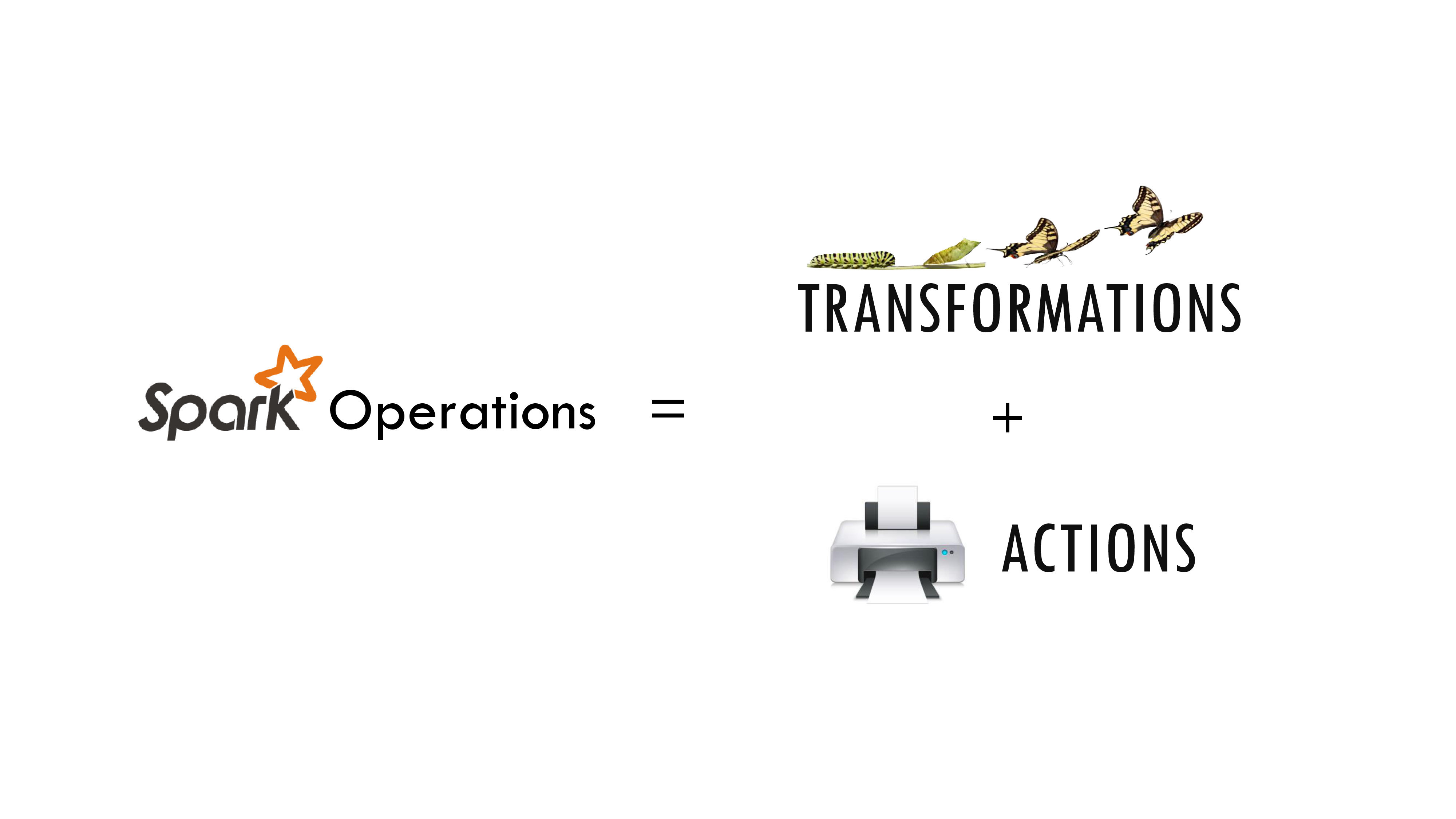
Once created, RDDs offer two types of operations: transformations and actions.
Read dataset from DataBase
## set up  SparkSession
from pyspark.sql import SparkSession

spark = SparkSession \
            .builder \
            .appName("Python Spark create RDD example") \
            .config("spark.some.config.option", "some-value") \
            .getOrCreate()

## User information
user = 'your_username'
pw   = 'your_password'

## Database information
table_name = 'table_name'
url = 'jdbc:postgresql://##.###.###.##:5432/dataset?user='+user+'&password='+pw
properties ={'driver': 'org.postgresql.Driver', 'password': pw,'user': user}

df = spark.read.jdbc(url=url, table=table_name, properties=properties)

df.show(5)
df.printSchema()
Then you will get the RDD data:
+---+-----+-----+---------+-----+
|_c0|   TV|Radio|Newspaper|Sales|
+---+-----+-----+---------+-----+
|  1|230.1| 37.8|     69.2| 22.1|
|  2| 44.5| 39.3|     45.1| 10.4|
|  3| 17.2| 45.9|     69.3|  9.3|
|  4|151.5| 41.3|     58.5| 18.5|
|  5|180.8| 10.8|     58.4| 12.9|
+---+-----+-----+---------+-----+
only showing top 5 rows

root
 |-- _c0: integer (nullable = true)
 |-- TV: double (nullable = true)
 |-- Radio: double (nullable = true)
 |-- Newspaper: double (nullable = true)
 |-- Sales: double (nullable = true)
Note
Reading tables from Database needs the proper drive for the corresponding Database.
For example, the above demo needs org.postgresql.Driver and you need to download
it and put it in jars folder of your spark installation path. I download
postgresql-42.1.1.jar from the official website and put it in jars folder.
Read dataset from HDFS
from pyspark.conf import SparkConf
from pyspark.context import SparkContext
from pyspark.sql import HiveContext

sc= SparkContext('local','example')
hc = HiveContext(sc)
tf1 = sc.textFile("hdfs://cdhstltest/user/data/demo.CSV")
print(tf1.first())

hc.sql("use intg_cme_w")
spf = hc.sql("SELECT * FROM spf LIMIT 100")
print(spf.show(5))
5.2. Spark Operations
Warning
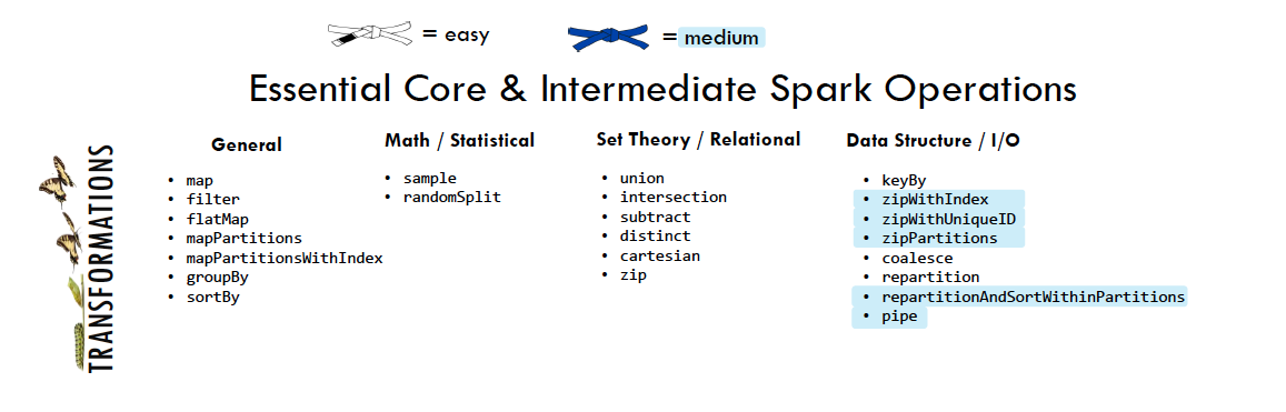
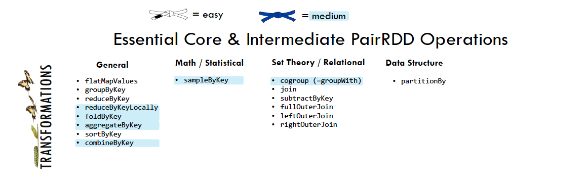
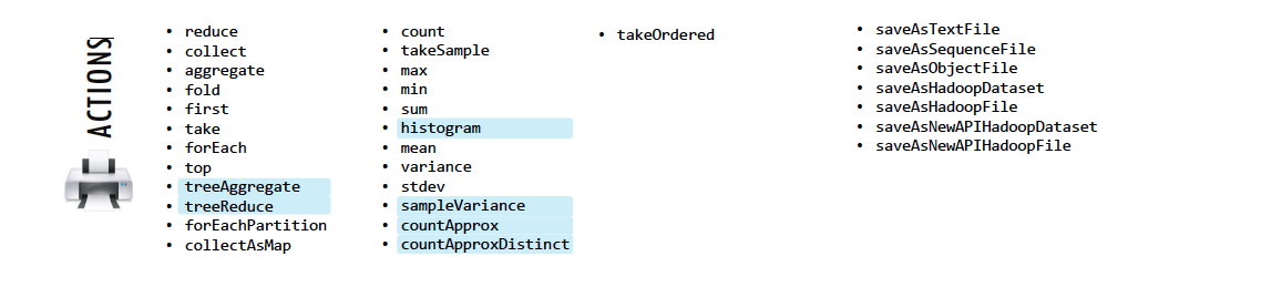
All the figures below are from Jeffrey Thompson. The interested reader is referred to pyspark pictures
There are two main types of Spark operations: Transformations and Actions [Karau2015].
Note
Some people defined three types of operations: Transformations, Actions and Shuffles.
5.2.1. Spark Transformations
Transformations construct a new RDD from a previous one. For example, one common transformation is filtering data that matches a predicate.
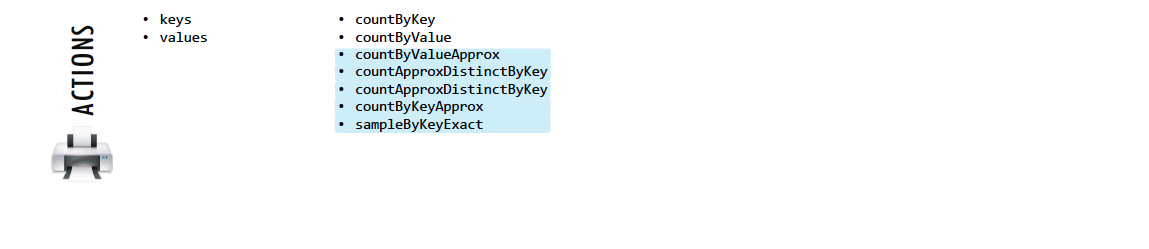
5.2.2. Spark Actions
Actions, on the other hand, compute a result based on an RDD, and either return it to the driver program or save it to an external storage system (e.g., HDFS).
5.3. rdd.DataFrame vs pd.DataFrame
5.3.1. Create DataFrame
From List
my_list = [['a', 1, 2], ['b', 2, 3],['c', 3, 4]]
col_name = ['A', 'B', 'C']
:: Python Code:
# caution for the columns=
pd.DataFrame(my_list,columns= col_name)
#
spark.createDataFrame(my_list, col_name).show()
:: Comparison:
                  +---+---+---+
                  |  A|  B|  C|
   A  B  C        +---+---+---+
0  a  1  2        |  a|  1|  2|
1  b  2  3        |  b|  2|  3|
2  c  3  4        |  c|  3|  4|
                  +---+---+---+
Attention
Pay attentation to the parameter columns= in pd.DataFrame. Since the default value will make the list as rows.
:: Python Code:# caution for the columns= pd.DataFrame(my_list, columns= col_name) # pd.DataFrame(my_list, col_name)
:: Comparison:A B C 0 1 2 0 a 1 2 A a 1 2 1 b 2 3 B b 2 3 2 c 3 4 C c 3 4
From Dict
d = {'A': [0, 1, 0],
     'B': [1, 0, 1],
     'C': [1, 0, 0]}
:: Python Code:
pd.DataFrame(d)for
# Tedious for PySpark
spark.createDataFrame(np.array(list(d.values())).T.tolist(),list(d.keys())).show()
:: Comparison:
                   +---+---+---+
                   |  A|  B|  C|
   A  B  C         +---+---+---+
0  0  1  1         |  0|  1|  1|
1  1  0  0         |  1|  0|  0|
2  0  1  0         |  0|  1|  0|
                   +---+---+---+
5.3.2. Load DataFrame
From DataBase
Most of time, you need to share your code with your colleagues or release your code for Code Review or Quality assurance(QA). You will definitely do not want to have your User Information in the code. So you can save them
in login.txt:
runawayhorse001
PythonTips
and use the following code to import your User Information:
#User Information
try:
    login = pd.read_csv(r'login.txt', header=None)
    user = login[0][0]
    pw = login[0][1]
    print('User information is ready!')
except:
    print('Login information is not available!!!')

#Database information
host = '##.###.###.##'
db_name = 'db_name'
table_name = 'table_name'
:: Comparison:
conn = psycopg2.connect(host=host, database=db_name, user=user, password=pw)
cur = conn.cursor()

sql = """
      select *
      from {table_name}
      """.format(table_name=table_name)
dp = pd.read_sql(sql, conn)
# connect to database
url = 'jdbc:postgresql://'+host+':5432/'+db_name+'?user='+user+'&password='+pw
properties ={'driver': 'org.postgresql.Driver', 'password': pw,'user': user}
ds = spark.read.jdbc(url=url, table=table_name, properties=properties)
Attention
Reading tables from Database with PySpark needs the proper drive for the corresponding Database. For example, the above demo needs org.postgresql.Driver and you need to download it and put it in jars folder of your spark installation path. I download postgresql-42.1.1.jar from the official website and put it in jars folder.
From
.csv
:: Comparison:
# pd.DataFrame dp: DataFrame pandas
dp = pd.read_csv('Advertising.csv')
#rdd.DataFrame. dp: DataFrame spark
ds = spark.read.csv(path='Advertising.csv',
#                sep=',',
#                encoding='UTF-8',
#                comment=None,
               header=True,
               inferSchema=True)
From
.json
Data from: http://api.luftdaten.info/static/v1/data.json
dp = pd.read_json("data/data.json")
ds = spark.read.json('data/data.json')
:: Python Code:
dp[['id','timestamp']].head(4)
#
ds[['id','timestamp']].show(4)
:: Comparison:
                                                +----------+-------------------+
                                                |        id|          timestamp|
            id  timestamp                       +----------+-------------------+
0   2994551481  2019-02-28 17:23:52             |2994551481|2019-02-28 17:23:52|
1   2994551482  2019-02-28 17:23:52             |2994551482|2019-02-28 17:23:52|
2   2994551483  2019-02-28 17:23:52             |2994551483|2019-02-28 17:23:52|
3   2994551484  2019-02-28 17:23:52             |2994551484|2019-02-28 17:23:52|
                                                +----------+-------------------+
                                                only showing top 4 rows
5.3.3. First n Rows
:: Python Code:
dp.head(4)
#
ds.show(4)
:: Comparison:
                                        +-----+-----+---------+-----+
                                        |   TV|Radio|Newspaper|Sales|
      TV  Radio  Newspaper  Sales       +-----+-----+---------+-----+
0  230.1   37.8       69.2   22.1       |230.1| 37.8|     69.2| 22.1|
1   44.5   39.3       45.1   10.4       | 44.5| 39.3|     45.1| 10.4|
2   17.2   45.9       69.3    9.3       | 17.2| 45.9|     69.3|  9.3|
3  151.5   41.3       58.5   18.5       |151.5| 41.3|     58.5| 18.5|
                                        +-----+-----+---------+-----+
                                        only showing top 4 rows
5.3.4. Column Names
:: Python Code:
dp.columns
#
ds.columns
:: Comparison:
Index(['TV', 'Radio', 'Newspaper', 'Sales'], dtype='object')
['TV', 'Radio', 'Newspaper', 'Sales']
5.3.5. Data types
:: Python Code:
dp.dtypes
#
ds.dtypes
:: Comparison:
TV           float64                    [('TV', 'double'),
Radio        float64                     ('Radio', 'double'),
Newspaper    float64                     ('Newspaper', 'double'),
Sales        float64                     ('Sales', 'double')]
dtype: object
5.3.6. Fill Null
my_list = [['male', 1, None], ['female', 2, 3],['male', 3, 4]]
dp = pd.DataFrame(my_list,columns=['A', 'B', 'C'])
ds = spark.createDataFrame(my_list, ['A', 'B', 'C'])
#
dp.head()
ds.show()
:: Comparison:
                                        +------+---+----+
                                        |     A|  B|   C|
        A  B    C                       +------+---+----+
0    male  1  NaN                       |  male|  1|null|
1  female  2  3.0                       |female|  2|   3|
2    male  3  4.0                       |  male|  3|   4|
                                        +------+---+----+
:: Python Code:
dp.fillna(-99)
#
ds.fillna(-99).show()
:: Comparison:
                                        +------+---+----+
                                        |     A|  B|   C|
        A  B    C                       +------+---+----+
0    male  1  -99                       |  male|  1| -99|
1  female  2  3.0                       |female|  2|   3|
2    male  3  4.0                       |  male|  3|   4|
                                        +------+---+----+
5.3.7. Replace Values
:: Python Code:
# caution: you need to chose specific col
dp.A.replace(['male', 'female'],[1, 0], inplace=True)
dp
#caution: Mixed type replacements are not supported
ds.na.replace(['male','female'],['1','0']).show()
:: Comparison:
                                +---+---+----+
                                |  A|  B|   C|
   A  B    C                    +---+---+----+
0  1  1  NaN                    |  1|  1|null|
1  0  2  3.0                    |  0|  2|   3|
2  1  3  4.0                    |  1|  3|   4|
                                +---+---+----+
5.3.8. Rename Columns
Rename all columns
:: Python Code:
dp.columns = ['a','b','c','d']
dp.head(4)
#
ds.toDF('a','b','c','d').show(4)
:: Comparison:
                                                +-----+----+----+----+
                                                |    a|   b|   c|   d|
       a     b     c     d                      +-----+----+----+----+
0  230.1  37.8  69.2  22.1                      |230.1|37.8|69.2|22.1|
1   44.5  39.3  45.1  10.4                      | 44.5|39.3|45.1|10.4|
2   17.2  45.9  69.3   9.3                      | 17.2|45.9|69.3| 9.3|
3  151.5  41.3  58.5  18.5                      |151.5|41.3|58.5|18.5|
                                                +-----+----+----+----+
                                                only showing top 4 rows
Rename one or more columns
mapping = {'Newspaper':'C','Sales':'D'}
:: Python Code:
dp.rename(columns=mapping).head(4)
#
new_names = [mapping.get(col,col) for col in ds.columns]
ds.toDF(*new_names).show(4)
:: Comparison:
                                        +-----+-----+----+----+
                                        |   TV|Radio|   C|   D|
      TV  Radio     C     D             +-----+-----+----+----+
0  230.1   37.8  69.2  22.1             |230.1| 37.8|69.2|22.1|
1   44.5   39.3  45.1  10.4             | 44.5| 39.3|45.1|10.4|
2   17.2   45.9  69.3   9.3             | 17.2| 45.9|69.3| 9.3|
3  151.5   41.3  58.5  18.5             |151.5| 41.3|58.5|18.5|
                                        +-----+-----+----+----+
                                        only showing top 4 rows
Note
You can also use withColumnRenamed to rename one column in PySpark.
:: Python Code:
ds.withColumnRenamed('Newspaper','Paper').show(4
:: Comparison:
+-----+-----+-----+-----+
|   TV|Radio|Paper|Sales|
+-----+-----+-----+-----+
|230.1| 37.8| 69.2| 22.1|
| 44.5| 39.3| 45.1| 10.4|
| 17.2| 45.9| 69.3|  9.3|
|151.5| 41.3| 58.5| 18.5|
+-----+-----+-----+-----+
only showing top 4 rows
5.3.9. Drop Columns
drop_name = ['Newspaper','Sales']
:: Python Code:
dp.drop(drop_name,axis=1).head(4)
#
ds.drop(*drop_name).show(4)
:: Comparison:
                                +-----+-----+
                                |   TV|Radio|
      TV  Radio                 +-----+-----+
0  230.1   37.8                 |230.1| 37.8|
1   44.5   39.3                 | 44.5| 39.3|
2   17.2   45.9                 | 17.2| 45.9|
3  151.5   41.3                 |151.5| 41.3|
                                +-----+-----+
                                only showing top 4 rows
5.3.10. Filter
dp = pd.read_csv('Advertising.csv')
#
ds = spark.read.csv(path='Advertising.csv',
                    header=True,
                    inferSchema=True)
:: Python Code:
dp[dp.Newspaper<20].head(4)
#
ds[ds.Newspaper<20].show(4)
:: Comparison:
                                                +-----+-----+---------+-----+
                                                |   TV|Radio|Newspaper|Sales|
       TV  Radio  Newspaper  Sales              +-----+-----+---------+-----+
7   120.2   19.6       11.6   13.2              |120.2| 19.6|     11.6| 13.2|
8     8.6    2.1        1.0    4.8              |  8.6|  2.1|      1.0|  4.8|
11  214.7   24.0        4.0   17.4              |214.7| 24.0|      4.0| 17.4|
13   97.5    7.6        7.2    9.7              | 97.5|  7.6|      7.2|  9.7|
                                                +-----+-----+---------+-----+
                                                only showing top 4 rows
:: Python Code:
dp[(dp.Newspaper<20)&(dp.TV>100)].head(4)
#
ds[(ds.Newspaper<20)&(ds.TV>100)].show(4)
:: Comparison:
                                                +-----+-----+---------+-----+
                                                |   TV|Radio|Newspaper|Sales|
       TV  Radio  Newspaper  Sales              +-----+-----+---------+-----+
7   120.2   19.6       11.6   13.2              |120.2| 19.6|     11.6| 13.2|
11  214.7   24.0        4.0   17.4              |214.7| 24.0|      4.0| 17.4|
19  147.3   23.9       19.1   14.6              |147.3| 23.9|     19.1| 14.6|
25  262.9    3.5       19.5   12.0              |262.9|  3.5|     19.5| 12.0|
                                                +-----+-----+---------+-----+
                                                only showing top 4 rows
5.3.11. With New Column
:: Python Code:
dp['tv_norm'] = dp.TV/sum(dp.TV)
dp.head(4)
#
ds.withColumn('tv_norm', ds.TV/ds.groupBy().agg(F.sum("TV")).collect()[0][0]).show(4)
:: Comparison:
                                                +-----+-----+---------+-----+--------------------+
                                                |   TV|Radio|Newspaper|Sales|             tv_norm|
      TV  Radio  Newspaper  Sales   tv_norm     +-----+-----+---------+-----+--------------------+
0  230.1   37.8       69.2   22.1  0.007824     |230.1| 37.8|     69.2| 22.1|0.007824268493802813|
1   44.5   39.3       45.1   10.4  0.001513     | 44.5| 39.3|     45.1| 10.4|0.001513167961643...|
2   17.2   45.9       69.3    9.3  0.000585     | 17.2| 45.9|     69.3|  9.3|5.848649200061207E-4|
3  151.5   41.3       58.5   18.5  0.005152     |151.5| 41.3|     58.5| 18.5|0.005151571824472517|
                                                +-----+-----+---------+-----+--------------------+
                                                only showing top 4 rows
:: Python Code:
dp['cond'] = dp.apply(lambda c: 1 if ((c.TV>100)&(c.Radio<40)) else 2 if c.Sales> 10 else 3,axis=1)
#
ds.withColumn('cond',F.when((ds.TV>100)&(ds.Radio<40),1)\
                      .when(ds.Sales>10, 2)\
                      .otherwise(3)).show(4)
:: Comparison:
                                                +-----+-----+---------+-----+----+
                                                |   TV|Radio|Newspaper|Sales|cond|
      TV  Radio  Newspaper  Sales  cond         +-----+-----+---------+-----+----+
0  230.1   37.8       69.2   22.1     1         |230.1| 37.8|     69.2| 22.1|   1|
1   44.5   39.3       45.1   10.4     2         | 44.5| 39.3|     45.1| 10.4|   2|
2   17.2   45.9       69.3    9.3     3         | 17.2| 45.9|     69.3|  9.3|   3|
3  151.5   41.3       58.5   18.5     2         |151.5| 41.3|     58.5| 18.5|   2|
                                                +-----+-----+---------+-----+----+
                                                only showing top 4 rows
:: Python Code:
dp['log_tv'] = np.log(dp.TV)
dp.head(4)
#
import pyspark.sql.functions as F
ds.withColumn('log_tv',F.log(ds.TV)).show(4)
:: Comparison:
                                                +-----+-----+---------+-----+------------------+
                                                |   TV|Radio|Newspaper|Sales|            log_tv|
      TV  Radio  Newspaper  Sales    log_tv     +-----+-----+---------+-----+------------------+
0  230.1   37.8       69.2   22.1  5.438514     |230.1| 37.8|     69.2| 22.1|  5.43851399704132|
1   44.5   39.3       45.1   10.4  3.795489     | 44.5| 39.3|     45.1| 10.4|3.7954891891721947|
2   17.2   45.9       69.3    9.3  2.844909     | 17.2| 45.9|     69.3|  9.3|2.8449093838194073|
3  151.5   41.3       58.5   18.5  5.020586     |151.5| 41.3|     58.5| 18.5| 5.020585624949423|
                                                +-----+-----+---------+-----+------------------+
                                                only showing top 4 rows
:: Python Code:
dp['tv+10'] = dp.TV.apply(lambda x: x+10)
dp.head(4)
#
ds.withColumn('tv+10', ds.TV+10).show(4)
:: Comparison:
                                                +-----+-----+---------+-----+-----+
                                                |   TV|Radio|Newspaper|Sales|tv+10|
      TV  Radio  Newspaper  Sales  tv+10        +-----+-----+---------+-----+-----+
0  230.1   37.8       69.2   22.1  240.1        |230.1| 37.8|     69.2| 22.1|240.1|
1   44.5   39.3       45.1   10.4   54.5        | 44.5| 39.3|     45.1| 10.4| 54.5|
2   17.2   45.9       69.3    9.3   27.2        | 17.2| 45.9|     69.3|  9.3| 27.2|
3  151.5   41.3       58.5   18.5  161.5        |151.5| 41.3|     58.5| 18.5|161.5|
                                                +-----+-----+---------+-----+-----+
                                                only showing top 4 rows
5.3.12. Join
leftp = pd.DataFrame({'A': ['A0', 'A1', 'A2', 'A3'],
                    'B': ['B0', 'B1', 'B2', 'B3'],
                    'C': ['C0', 'C1', 'C2', 'C3'],
                    'D': ['D0', 'D1', 'D2', 'D3']},
                    index=[0, 1, 2, 3])

rightp = pd.DataFrame({'A': ['A0', 'A1', 'A6', 'A7'],
                       'F': ['B4', 'B5', 'B6', 'B7'],
                       'G': ['C4', 'C5', 'C6', 'C7'],
                       'H': ['D4', 'D5', 'D6', 'D7']},
                       index=[4, 5, 6, 7])

lefts = spark.createDataFrame(leftp)
rights = spark.createDataFrame(rightp)
    A   B   C   D                   A   F   G   H
0  A0  B0  C0  D0               4  A0  B4  C4  D4
1  A1  B1  C1  D1               5  A1  B5  C5  D5
2  A2  B2  C2  D2               6  A6  B6  C6  D6
3  A3  B3  C3  D3               7  A7  B7  C7  D7
Left Join
:: Python Code:leftp.merge(rightp,on='A',how='left') # lefts.join(rights,on='A',how='left') .orderBy('A',ascending=True).show()
:: Comparison:+---+---+---+---+----+----+----+ | A| B| C| D| F| G| H| A B C D F G H +---+---+---+---+----+----+----+ 0 A0 B0 C0 D0 B4 C4 D4 | A0| B0| C0| D0| B4| C4| D4| 1 A1 B1 C1 D1 B5 C5 D5 | A1| B1| C1| D1| B5| C5| D5| 2 A2 B2 C2 D2 NaN NaN NaN | A2| B2| C2| D2|null|null|null| 3 A3 B3 C3 D3 NaN NaN NaN | A3| B3| C3| D3|null|null|null| +---+---+---+---+----+----+----+
Right Join
:: Python Code:leftp.merge(rightp,on='A',how='right') # lefts.join(rights,on='A',how='right') .orderBy('A',ascending=True).show()
:: Comparison:+---+----+----+----+---+---+---+ | A| B| C| D| F| G| H| A B C D F G H +---+----+----+----+---+---+---+ 0 A0 B0 C0 D0 B4 C4 D4 | A0| B0| C0| D0| B4| C4| D4| 1 A1 B1 C1 D1 B5 C5 D5 | A1| B1| C1| D1| B5| C5| D5| 2 A6 NaN NaN NaN B6 C6 D6 | A6|null|null|null| B6| C6| D6| 3 A7 NaN NaN NaN B7 C7 D7 | A7|null|null|null| B7| C7| D7| +---+----+----+----+---+---+---+
Inner Join
:: Python Code:leftp.merge(rightp,on='A',how='inner') # lefts.join(rights,on='A',how='inner') .orderBy('A',ascending=True).show()
:: Comparison:+---+---+---+---+---+---+---+ | A| B| C| D| F| G| H| A B C D F G H +---+---+---+---+---+---+---+ 0 A0 B0 C0 D0 B4 C4 D4 | A0| B0| C0| D0| B4| C4| D4| 1 A1 B1 C1 D1 B5 C5 D5 | A1| B1| C1| D1| B5| C5| D5| +---+---+---+---+---+---+---+
Full Join
:: Python Code:leftp.merge(rightp,on='A',how='outer') # lefts.join(rights,on='A',how='full') .orderBy('A',ascending=True).show()
:: Comparison:+---+----+----+----+----+----+----+ | A| B| C| D| F| G| H| A B C D F G H +---+----+----+----+----+----+----+ 0 A0 B0 C0 D0 B4 C4 D4 | A0| B0| C0| D0| B4| C4| D4| 1 A1 B1 C1 D1 B5 C5 D5 | A1| B1| C1| D1| B5| C5| D5| 2 A2 B2 C2 D2 NaN NaN NaN | A2| B2| C2| D2|null|null|null| 3 A3 B3 C3 D3 NaN NaN NaN | A3| B3| C3| D3|null|null|null| 4 A6 NaN NaN NaN B6 C6 D6 | A6|null|null|null| B6| C6| D6| 5 A7 NaN NaN NaN B7 C7 D7 | A7|null|null|null| B7| C7| D7| +---+----+----+----+----+----+----+
5.3.13. Concat Columns
my_list = [('a', 2, 3),
           ('b', 5, 6),
           ('c', 8, 9),
           ('a', 2, 3),
           ('b', 5, 6),
           ('c', 8, 9)]
col_name = ['col1', 'col2', 'col3']
#
dp = pd.DataFrame(my_list,columns=col_name)
ds = spark.createDataFrame(my_list,schema=col_name)
  col1  col2  col3
0    a     2     3
1    b     5     6
2    c     8     9
3    a     2     3
4    b     5     6
5    c     8     9
:: Python Code:
dp['concat'] = dp.apply(lambda x:'%s%s'%(x['col1'],x['col2']),axis=1)
dp
#
ds.withColumn('concat',F.concat('col1','col2')).show()
:: Comparison:
                                        +----+----+----+------+
                                        |col1|col2|col3|concat|
  col1  col2  col3 concat               +----+----+----+------+
0    a     2     3     a2               |   a|   2|   3|    a2|
1    b     5     6     b5               |   b|   5|   6|    b5|
2    c     8     9     c8               |   c|   8|   9|    c8|
3    a     2     3     a2               |   a|   2|   3|    a2|
4    b     5     6     b5               |   b|   5|   6|    b5|
5    c     8     9     c8               |   c|   8|   9|    c8|
                                        +----+----+----+------+
5.3.14. GroupBy
:: Python Code:
dp.groupby(['col1']).agg({'col2':'min','col3':'mean'})
#
ds.groupBy(['col1']).agg({'col2': 'min', 'col3': 'avg'}).show()
:: Comparison:
                                        +----+---------+---------+
      col2  col3                        |col1|min(col2)|avg(col3)|
col1                                    +----+---------+---------+
a        2     3                        |   c|        8|      9.0|
b        5     6                        |   b|        5|      6.0|
c        8     9                        |   a|        2|      3.0|
                                        +----+---------+---------+
5.3.15. Pivot
:: Python Code:
pd.pivot_table(dp, values='col3', index='col1', columns='col2', aggfunc=np.sum)
#
ds.groupBy(['col1']).pivot('col2').sum('col3').show()
:: Comparison:
                                +----+----+----+----+
col2    2     5     8           |col1|   2|   5|   8|
col1                            +----+----+----+----+
a     6.0   NaN   NaN           |   c|null|null|  18|
b     NaN  12.0   NaN           |   b|null|  12|null|
c     NaN   NaN  18.0           |   a|   6|null|null|
                                +----+----+----+----+
5.3.16. Window
d = {'A':['a','b','c','d'],'B':['m','m','n','n'],'C':[1,2,3,6]}
dp = pd.DataFrame(d)
ds = spark.createDataFrame(dp)
:: Python Code:
dp['rank'] = dp.groupby('B')['C'].rank('dense',ascending=False)
#
from pyspark.sql.window import Window
w = Window.partitionBy('B').orderBy(ds.C.desc())
ds = ds.withColumn('rank',F.rank().over(w))
:: Comparison:
                        +---+---+---+----+
                        |  A|  B|  C|rank|
   A  B  C  rank        +---+---+---+----+
0  a  m  1   2.0        |  b|  m|  2|   1|
1  b  m  2   1.0        |  a|  m|  1|   2|
2  c  n  3   2.0        |  d|  n|  6|   1|
3  d  n  6   1.0        |  c|  n|  3|   2|
                        +---+---+---+----+
5.3.17. rank vs dense_rank
d ={'Id':[1,2,3,4,5,6],
    'Score': [4.00, 4.00, 3.85, 3.65, 3.65, 3.50]}
#
data = pd.DataFrame(d)
dp = data.copy()
ds = spark.createDataFrame(data)
   Id  Score
0   1   4.00
1   2   4.00
2   3   3.85
3   4   3.65
4   5   3.65
5   6   3.50
:: Python Code:
dp['Rank_dense'] = dp['Score'].rank(method='dense',ascending =False)
dp['Rank'] = dp['Score'].rank(method='min',ascending =False)
dp
#
import pyspark.sql.functions as F
from pyspark.sql.window import Window
w = Window.orderBy(ds.Score.desc())
ds = ds.withColumn('Rank_spark_dense',F.dense_rank().over(w))
ds = ds.withColumn('Rank_spark',F.rank().over(w))
ds.show()
:: Comparison:
                                +---+-----+----------------+----------+
                                | Id|Score|Rank_spark_dense|Rank_spark|
   Id  Score  Rank_dense  Rank  +---+-----+----------------+----------+
0   1   4.00         1.0   1.0  |  1|  4.0|               1|         1|
1   2   4.00         1.0   1.0  |  2|  4.0|               1|         1|
2   3   3.85         2.0   3.0  |  3| 3.85|               2|         3|
3   4   3.65         3.0   4.0  |  4| 3.65|               3|         4|
4   5   3.65         3.0   4.0  |  5| 3.65|               3|         4|
5   6   3.50         4.0   6.0  |  6|  3.5|               4|         6|
                                +---+-----+----------------+----------+