13. RFM Analysis
The above figure source: Blast Analytics Marketing
RFM is a method used for analyzing customer value. It is commonly used in database marketing and direct marketing and has received particular attention in retail and professional services industries. More details can be found at Wikipedia RFM_wikipedia.
RFM stands for the three dimensions:
Recency – How recently did the customer purchase? i.e. Duration since last purchase
Frequency – How often do they purchase? i.e. Total number of purchases
Monetary Value – How much do they spend? i.e. Total money this customer spent
13.1. RFM Analysis Methodology
RFM Analysis contains three main steps:
13.1.1. 1. Build the RFM features matrix for each customer
+----------+-------+---------+---------+
|CustomerID|Recency|Frequency| Monetary|
+----------+-------+---------+---------+
|     14911|      1|      248|132572.62|
|     12748|      0|      224|  29072.1|
|     17841|      1|      169| 40340.78|
|     14606|      1|      128| 11713.85|
|     15311|      0|      118| 59419.34|
+----------+-------+---------+---------+
only showing top 5 rows
13.1.2. 2. Determine cutting points for each feature
+----------+-------+---------+--------+-----+-----+-----+
|CustomerID|Recency|Frequency|Monetary|r_seg|f_seg|m_seg|
+----------+-------+---------+--------+-----+-----+-----+
|     17420|     50|        3|  598.83|    2|    3|    2|
|     16861|     59|        3|  151.65|    3|    3|    1|
|     16503|    106|        5| 1421.43|    3|    2|    3|
|     15727|     16|        7| 5178.96|    1|    1|    4|
|     17389|      0|       43|31300.08|    1|    1|    4|
+----------+-------+---------+--------+-----+-----+-----+
only showing top 5 rows
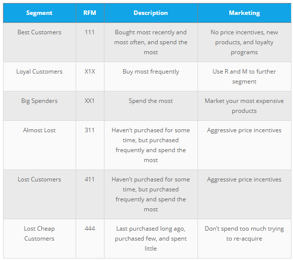
13.1.3. 3. Determine the RFM scores and summarize the corresponding business value
+----------+-------+---------+--------+-----+-----+-----+--------+
|CustomerID|Recency|Frequency|Monetary|r_seg|f_seg|m_seg|RFMScore|
+----------+-------+---------+--------+-----+-----+-----+--------+
|     17988|     11|        8|  191.17|    1|    1|    1|     111|
|     16892|      1|        7|  496.84|    1|    1|    2|     112|
|     16668|     15|        6|  306.72|    1|    1|    2|     112|
|     16554|      3|        7|  641.55|    1|    1|    2|     112|
|     16500|      4|        6|  400.86|    1|    1|    2|     112|
+----------+-------+---------+--------+-----+-----+-----+--------+
only showing top 5 rows
The corresponding business description and marketing value:
Source: Blast Analytics Marketing
13.2. Demo
The Jupyter notebook can be download from Data Exploration.
The data can be downloaf from German Credit.
13.2.1. Load and clean data
Set up spark context and SparkSession
from pyspark.sql import SparkSession

spark = SparkSession \
    .builder \
    .appName("Python Spark RFM example") \
    .config("spark.some.config.option", "some-value") \
    .getOrCreate()
Load dataset
df_raw = spark.read.format('com.databricks.spark.csv').\
                       options(header='true', \
                       inferschema='true').\
            load("Online Retail.csv",header=True);
check the data set
df_raw.show(5)
df_raw.printSchema()
Then you will get
+---------+---------+--------------------+--------+------------+---------+----------+--------------+
|InvoiceNo|StockCode|         Description|Quantity| InvoiceDate|UnitPrice|CustomerID|       Country|
+---------+---------+--------------------+--------+------------+---------+----------+--------------+
|   536365|   85123A|WHITE HANGING HEA...|       6|12/1/10 8:26|     2.55|     17850|United Kingdom|
|   536365|    71053| WHITE METAL LANTERN|       6|12/1/10 8:26|     3.39|     17850|United Kingdom|
|   536365|   84406B|CREAM CUPID HEART...|       8|12/1/10 8:26|     2.75|     17850|United Kingdom|
|   536365|   84029G|KNITTED UNION FLA...|       6|12/1/10 8:26|     3.39|     17850|United Kingdom|
|   536365|   84029E|RED WOOLLY HOTTIE...|       6|12/1/10 8:26|     3.39|     17850|United Kingdom|
+---------+---------+--------------------+--------+------------+---------+----------+--------------+
only showing top 5 rows

root
 |-- InvoiceNo: string (nullable = true)
 |-- StockCode: string (nullable = true)
 |-- Description: string (nullable = true)
 |-- Quantity: integer (nullable = true)
 |-- InvoiceDate: string (nullable = true)
 |-- UnitPrice: double (nullable = true)
 |-- CustomerID: integer (nullable = true)
 |-- Country: string (nullable = true)
Data clean and data manipulation
check and remove the
nullvalues
from pyspark.sql.functions import count

def my_count(df_in):
    df_in.agg( *[ count(c).alias(c) for c in df_in.columns ] ).show()
my_count(df_raw)
+---------+---------+-----------+--------+-----------+---------+----------+-------+
|InvoiceNo|StockCode|Description|Quantity|InvoiceDate|UnitPrice|CustomerID|Country|
+---------+---------+-----------+--------+-----------+---------+----------+-------+
|   541909|   541909|     540455|  541909|     541909|   541909|    406829| 541909|
+---------+---------+-----------+--------+-----------+---------+----------+-------+
Since the count results are not the same, we have some null value in the CustomerID column. We can drop these records from the dataset.
df = df_raw.dropna(how='any')
my_count(df)
+---------+---------+-----------+--------+-----------+---------+----------+-------+
|InvoiceNo|StockCode|Description|Quantity|InvoiceDate|UnitPrice|CustomerID|Country|
+---------+---------+-----------+--------+-----------+---------+----------+-------+
|   406829|   406829|     406829|  406829|     406829|   406829|    406829| 406829|
+---------+---------+-----------+--------+-----------+---------+----------+-------+
Dealwith the InvoiceDate
from pyspark.sql.functions import to_utc_timestamp, unix_timestamp, lit, datediff, col

timeFmt = "MM/dd/yy HH:mm"

df = df.withColumn('NewInvoiceDate'
                 , to_utc_timestamp(unix_timestamp(col('InvoiceDate'),timeFmt).cast('timestamp')
                 , 'UTC'))
df.show(5)

+---------+---------+--------------------+--------+------------+---------+----------+--------------+--------------------+
|InvoiceNo|StockCode|         Description|Quantity| InvoiceDate|UnitPrice|CustomerID|       Country|      NewInvoiceDate|
+---------+---------+--------------------+--------+------------+---------+----------+--------------+--------------------+
|   536365|   85123A|WHITE HANGING HEA...|       6|12/1/10 8:26|     2.55|     17850|United Kingdom|2010-12-01 08:26:...|
|   536365|    71053| WHITE METAL LANTERN|       6|12/1/10 8:26|     3.39|     17850|United Kingdom|2010-12-01 08:26:...|
|   536365|   84406B|CREAM CUPID HEART...|       8|12/1/10 8:26|     2.75|     17850|United Kingdom|2010-12-01 08:26:...|
|   536365|   84029G|KNITTED UNION FLA...|       6|12/1/10 8:26|     3.39|     17850|United Kingdom|2010-12-01 08:26:...|
|   536365|   84029E|RED WOOLLY HOTTIE...|       6|12/1/10 8:26|     3.39|     17850|United Kingdom|2010-12-01 08:26:...|
+---------+---------+--------------------+--------+------------+---------+----------+--------------+--------------------+
only showing top 5 rows
Warning
The spark is pretty sensitive to the date format!
calculate total price
from pyspark.sql.functions import round

df = df.withColumn('TotalPrice', round( df.Quantity * df.UnitPrice, 2 ) )
calculate the time difference
from pyspark.sql.functions import mean, min, max, sum, datediff, to_date

date_max = df.select(max('NewInvoiceDate')).toPandas()
current = to_utc_timestamp( unix_timestamp(lit(str(date_max.iloc[0][0])), \
                              'yy-MM-dd HH:mm').cast('timestamp'), 'UTC' )

# Calculatre Duration
df = df.withColumn('Duration', datediff(lit(current), 'NewInvoiceDate'))
build the Recency, Frequency and Monetary
recency = df.groupBy('CustomerID').agg(min('Duration').alias('Recency'))
frequency = df.groupBy('CustomerID', 'InvoiceNo').count()\
                        .groupBy('CustomerID')\
                        .agg(count("*").alias("Frequency"))
monetary = df.groupBy('CustomerID').agg(round(sum('TotalPrice'), 2).alias('Monetary'))
rfm = recency.join(frequency,'CustomerID', how = 'inner')\
             .join(monetary,'CustomerID', how = 'inner')
rfm.show(5)

+----------+-------+---------+--------+
|CustomerID|Recency|Frequency|Monetary|
+----------+-------+---------+--------+
|     17420|     50|        3|  598.83|
|     16861|     59|        3|  151.65|
|     16503|    106|        5| 1421.43|
|     15727|     16|        7| 5178.96|
|     17389|      0|       43|31300.08|
+----------+-------+---------+--------+
only showing top 5 rows
13.2.2. RFM Segmentation
Determine cutting points
In this section, you can use the techniques (statistical results and visualizations) in Data Exploration section to help you determine the cutting points for each attribute. In my opinion, the cutting points are mainly depend on the business sense. You’s better talk to your makrting people and get feedback and suggestion from them. I will use the quantile as the cutting points in this demo.
cols = ['Recency','Frequency','Monetary']
describe_pd(rfm,cols,1)
+-------+-----------------+-----------------+------------------+
|summary|          Recency|        Frequency|          Monetary|
+-------+-----------------+-----------------+------------------+
|  count|           4372.0|           4372.0|            4372.0|
|   mean|91.58119853613907| 5.07548032936871|1898.4597003659655|
| stddev|100.7721393138483|9.338754163574727| 8219.345141139722|
|    min|              0.0|              1.0|          -4287.63|
|    max|            373.0|            248.0|         279489.02|
|    25%|             16.0|              1.0|293.36249999999995|
|    50%|             50.0|              3.0|           648.075|
|    75%|            143.0|              5.0|          1611.725|
+-------+-----------------+-----------------+------------------+
The user defined function by using the cutting points:
def RScore(x):
    if  x <= 16:
        return 1
    elif x<= 50:
        return 2
    elif x<= 143:
        return 3
    else:
        return 4

def FScore(x):
    if  x <= 1:
        return 4
    elif x <= 3:
        return 3
    elif x <= 5:
        return 2
    else:
        return 1

def MScore(x):
    if  x <= 293:
        return 4
    elif x <= 648:
        return 3
    elif x <= 1611:
        return 2
    else:
        return 1

from pyspark.sql.functions import udf
from pyspark.sql.types import StringType, DoubleType

R_udf = udf(lambda x: RScore(x), StringType())
F_udf = udf(lambda x: FScore(x), StringType())
M_udf = udf(lambda x: MScore(x), StringType())
RFM Segmentation
rfm_seg = rfm.withColumn("r_seg", R_udf("Recency"))
rfm_seg = rfm_seg.withColumn("f_seg", F_udf("Frequency"))
rfm_seg = rfm_seg.withColumn("m_seg", M_udf("Monetary"))
rfm_seg.show(5)
+----------+-------+---------+--------+-----+-----+-----+
|CustomerID|Recency|Frequency|Monetary|r_seg|f_seg|m_seg|
+----------+-------+---------+--------+-----+-----+-----+
|     17420|     50|        3|  598.83|    2|    3|    2|
|     16861|     59|        3|  151.65|    3|    3|    1|
|     16503|    106|        5| 1421.43|    3|    2|    3|
|     15727|     16|        7| 5178.96|    1|    1|    4|
|     17389|      0|       43|31300.08|    1|    1|    4|
+----------+-------+---------+--------+-----+-----+-----+
only showing top 5 rows
rfm_seg = rfm_seg.withColumn('RFMScore',
                             F.concat(F.col('r_seg'),F.col('f_seg'), F.col('m_seg')))
rfm_seg.sort(F.col('RFMScore')).show(5)
+----------+-------+---------+--------+-----+-----+-----+--------+
|CustomerID|Recency|Frequency|Monetary|r_seg|f_seg|m_seg|RFMScore|
+----------+-------+---------+--------+-----+-----+-----+--------+
|     17988|     11|        8|  191.17|    1|    1|    1|     111|
|     16892|      1|        7|  496.84|    1|    1|    2|     112|
|     16668|     15|        6|  306.72|    1|    1|    2|     112|
|     16554|      3|        7|  641.55|    1|    1|    2|     112|
|     16500|      4|        6|  400.86|    1|    1|    2|     112|
+----------+-------+---------+--------+-----+-----+-----+--------+
only showing top 5 rows
13.2.3. Statistical Summary
Statistical Summary
simple summary
rfm_seg.groupBy('RFMScore')\
       .agg({'Recency':'mean',
             'Frequency': 'mean',
             'Monetary': 'mean'} )\
        .sort(F.col('RFMScore')).show(5)
+--------+-----------------+------------------+------------------+
|RFMScore|     avg(Recency)|     avg(Monetary)|    avg(Frequency)|
+--------+-----------------+------------------+------------------+
|     111|             11.0|            191.17|               8.0|
|     112|              8.0|          505.9775|               7.5|
|     113|7.237113402061856|1223.3604123711339| 7.752577319587629|
|     114|6.035123966942149| 8828.888595041324|18.882231404958677|
|     121|              9.6|            207.24|               4.4|
+--------+-----------------+------------------+------------------+
only showing top 5 rows
complex summary
grp = 'RFMScore'
num_cols = ['Recency','Frequency','Monetary']
df_input = rfm_seg

quantile_grouped = quantile_agg(df_input,grp,num_cols)
quantile_grouped.toPandas().to_csv(output_dir+'quantile_grouped.csv')

deciles_grouped = deciles_agg(df_input,grp,num_cols)
deciles_grouped.toPandas().to_csv(output_dir+'deciles_grouped.csv')
13.3. Extension
You can also apply the K-means clustering in Clustering section to do the segmentation.
13.3.1. Build feature matrix
build dense feature matrix
from pyspark.sql import Row
from pyspark.ml.linalg import Vectors

# method 1 (good for small feature):
#def transData(row):
#    return Row(label=row["Sales"],
#               features=Vectors.dense([row["TV"],
#                                       row["Radio"],
#                                       row["Newspaper"]]))

# Method 2 (good for large features):
def transData(data):
    return data.rdd.map(lambda r: [r[0],Vectors.dense(r[1:])]).toDF(['CustomerID','rfm'])
transformed= transData(rfm)
transformed.show(5)
+----------+-------------------+
|CustomerID|                rfm|
+----------+-------------------+
|     17420|  [50.0,3.0,598.83]|
|     16861|  [59.0,3.0,151.65]|
|     16503|[106.0,5.0,1421.43]|
|     15727| [16.0,7.0,5178.96]|
|     17389|[0.0,43.0,31300.08]|
+----------+-------------------+
only showing top 5 rows
Scaler the feature matrix
from pyspark.ml.feature import MinMaxScaler

scaler = MinMaxScaler(inputCol="rfm",\
         outputCol="features")
scalerModel =  scaler.fit(transformed)
scaledData = scalerModel.transform(transformed)
scaledData.show(5,False)
+----------+-------------------+--------------------------------------------------------------+
|CustomerID|rfm                |features                                                      |
+----------+-------------------+--------------------------------------------------------------+
|17420     |[50.0,3.0,598.83]  |[0.13404825737265416,0.008097165991902834,0.01721938714830836]|
|16861     |[59.0,3.0,151.65]  |[0.1581769436997319,0.008097165991902834,0.01564357039241953] |
|16503     |[106.0,5.0,1421.43]|[0.28418230563002683,0.016194331983805668,0.02011814573186342]|
|15727     |[16.0,7.0,5178.96] |[0.04289544235924933,0.024291497975708502,0.03335929858922501]|
|17389     |[0.0,43.0,31300.08]|[0.0,0.1700404858299595,0.12540746393334334]                  |
+----------+-------------------+--------------------------------------------------------------+
only showing top 5 rows
13.3.2. K-means clustering
Find optimal number of cluster
I will present two popular ways to determine the optimal number of the cluster.
elbow analysis
#PySpark libraries
from pyspark.ml import Pipeline
from pyspark.ml.feature import StringIndexer, OneHotEncoder, VectorAssembler
from pyspark.sql.functions import col, percent_rank, lit
from pyspark.sql.window import Window
from pyspark.sql import DataFrame, Row
from pyspark.sql.types import StructType
from functools import reduce  # For Python 3.x

from pyspark.ml.clustering import KMeans
#from pyspark.ml.evaluation import ClusteringEvaluator  # requires Spark 2.4 or later

import numpy as np
cost = np.zeros(20)
for k in range(2,20):
    kmeans = KMeans()\
            .setK(k)\
            .setSeed(1) \
            .setFeaturesCol("features")\
            .setPredictionCol("cluster")

    model = kmeans.fit(scaledData)
    cost[k] = model.computeCost(scaledData) # requires Spark 2.0 or later
import numpy as np
import matplotlib.mlab as mlab
import matplotlib.pyplot as plt
import seaborn as sbs
from matplotlib.ticker import MaxNLocator

fig, ax = plt.subplots(1,1, figsize =(8,6))
ax.plot(range(2,20),cost[2:20], marker = "o")
ax.set_xlabel('k')
ax.set_ylabel('cost')
ax.xaxis.set_major_locator(MaxNLocator(integer=True))
plt.show()
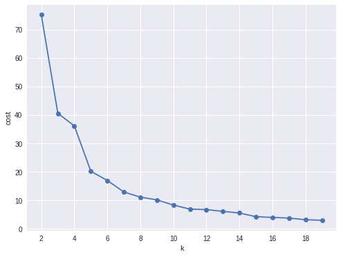
Cost v.s. the number of the clusters
In my opinion, sometimes it’s hard to choose the number of the clusters. As shown in Figure Cost v.s. the number of the clusters, you can choose 3, 5 or even 8. I will choose 3 in this demo.
Silhouette analysis
#PySpark libraries
from pyspark.ml import Pipeline
from pyspark.ml.feature import StringIndexer, OneHotEncoder, VectorAssembler
from pyspark.sql.functions import col, percent_rank, lit
from pyspark.sql.window import Window
from pyspark.sql import DataFrame, Row
from pyspark.sql.types import StructType
from functools import reduce  # For Python 3.x

from pyspark.ml.clustering import KMeans
from pyspark.ml.evaluation import ClusteringEvaluator

def optimal_k(df_in,index_col,k_min, k_max,num_runs):
    '''
    Determine optimal number of clusters by using Silhoutte Score Analysis.
    :param df_in: the input dataframe
    :param index_col: the name of the index column
    :param k_min: the train dataset
    :param k_min: the minmum number of the clusters
    :param k_max: the maxmum number of the clusters
    :param num_runs: the number of runs for each fixed clusters

    :return k: optimal number of the clusters
    :return silh_lst: Silhouette score
    :return r_table: the running results table

    :author: Wenqiang Feng
    :email:  von198@gmail.com.com
    '''

    start = time.time()
    silh_lst = []
    k_lst = np.arange(k_min, k_max+1)

    r_table = df_in.select(index_col).toPandas()
    r_table = r_table.set_index(index_col)
    centers = pd.DataFrame()

    for k in k_lst:
        silh_val = []
        for run in np.arange(1, num_runs+1):

            # Trains a k-means model.
            kmeans = KMeans()\
                    .setK(k)\
                    .setSeed(int(np.random.randint(100, size=1)))
            model = kmeans.fit(df_in)

            # Make predictions
            predictions = model.transform(df_in)
            r_table['cluster_{k}_{run}'.format(k=k, run=run)]= predictions.select('prediction').toPandas()

            # Evaluate clustering by computing Silhouette score
            evaluator = ClusteringEvaluator()
            silhouette = evaluator.evaluate(predictions)
            silh_val.append(silhouette)

        silh_array=np.asanyarray(silh_val)
        silh_lst.append(silh_array.mean())

    elapsed =  time.time() - start

    silhouette = pd.DataFrame(list(zip(k_lst,silh_lst)),columns = ['k', 'silhouette'])

    print('+------------------------------------------------------------+')
    print("|         The finding optimal k phase took %8.0f s.       |" %(elapsed))
    print('+------------------------------------------------------------+')


    return k_lst[np.argmax(silh_lst, axis=0)], silhouette , r_table
k, silh_lst, r_table = optimal_k(scaledData,index_col,k_min, k_max,num_runs)

+------------------------------------------------------------+
|         The finding optimal k phase took     1783 s.       |
+------------------------------------------------------------+
spark.createDataFrame(silh_lst).show()

+---+------------------+
|  k|        silhouette|
+---+------------------+
|  3|0.8045154385557953|
|  4|0.6993528775512052|
|  5|0.6689286654221447|
|  6|0.6356184024841809|
|  7|0.7174102265711756|
|  8|0.6720861758298997|
|  9| 0.601771359881241|
| 10|0.6292447334578428|
+---+------------------+
From the silhouette list, we can choose 3 as the optimal number of the clusters.
Warning
ClusteringEvaluator in pyspark.ml.evaluation requires Spark 2.4 or later!!
K-means clustering
k = 3
kmeans = KMeans().setK(k).setSeed(1)
model = kmeans.fit(scaledData)
# Make predictions
predictions = model.transform(scaledData)
predictions.show(5,False)
+----------+-------------------+--------------------+----------+
|CustomerID|                rfm|            features|prediction|
+----------+-------------------+--------------------+----------+
|     17420|  [50.0,3.0,598.83]|[0.13404825737265...|         0|
|     16861|  [59.0,3.0,151.65]|[0.15817694369973...|         0|
|     16503|[106.0,5.0,1421.43]|[0.28418230563002...|         2|
|     15727| [16.0,7.0,5178.96]|[0.04289544235924...|         0|
|     17389|[0.0,43.0,31300.08]|[0.0,0.1700404858...|         0|
+----------+-------------------+--------------------+----------+
only showing top 5 rows
13.3.3. Statistical summary
statistical summary
results = rfm.join(predictions.select('CustomerID','prediction'),'CustomerID',how='left')
results.show(5)
+----------+-------+---------+--------+----------+
|CustomerID|Recency|Frequency|Monetary|prediction|
+----------+-------+---------+--------+----------+
|     13098|      1|       41|28658.88|         0|
|     13248|    124|        2|  465.68|         2|
|     13452|    259|        2|   590.0|         1|
|     13460|     29|        2|  183.44|         0|
|     13518|     85|        1|  659.44|         0|
+----------+-------+---------+--------+----------+
only showing top 5 rows
simple summary
results.groupBy('prediction')\
       .agg({'Recency':'mean',
             'Frequency': 'mean',
             'Monetary': 'mean'} )\
        .sort(F.col('prediction')).show(5)
+----------+------------------+------------------+------------------+
|prediction|      avg(Recency)|     avg(Monetary)|    avg(Frequency)|
+----------+------------------+------------------+------------------+
|         0|30.966337980278816|2543.0355321319284| 6.514450867052023|
|         1|296.02403846153845|407.16831730769206|1.5592948717948718|
|         2|154.40148698884758| 702.5096406443623| 2.550185873605948|
+----------+------------------+------------------+------------------+
complex summary
grp = 'RFMScore'
num_cols = ['Recency','Frequency','Monetary']
df_input = results

quantile_grouped = quantile_agg(df_input,grp,num_cols)
quantile_grouped.toPandas().to_csv(output_dir+'quantile_grouped.csv')

deciles_grouped = deciles_agg(df_input,grp,num_cols)
deciles_grouped.toPandas().to_csv(output_dir+'deciles_grouped.csv')