require package
library(plyr)
library(asbio)
Load data
dt <- read.table("./data/CH22PR11.txt",
                col.names =  c("physical_therapy_days", "fitness_status", "obs", "age"))

dt$fitness_status = as.factor(dt$fitness_status)
dt$obs = as.factor(dt$obs)
Problem a
Test residuals normality
- W = 0.98277, p-value = 0.9409
- Normality test indicates that the residuals are normally distributed
fit = aov(physical_therapy_days~age+fitness_status, dt)
shapiro.test(fit$residuals)
##
##  Shapiro-Wilk normality test
##
## data:  fit$residuals
## W = 0.98277, p-value = 0.9409
Problem b
interaction between treatment factor and covariate
- F_star = 0.3359, P value = 0.719
- So no interaction between factor and covariate
fit.interaction = aov(physical_therapy_days~age+fitness_status+age:fitness_status, dt)
summary(fit.interaction)
##                    Df Sum Sq Mean Sq  F value   Pr(>F)
## age                 1  835.8   835.8 2530.910  < 2e-16 ***
## fitness_status      2  246.1   123.0  372.609 2.26e-15 ***
## age:fitness_status  2    0.2     0.1    0.336    0.719
## Residuals          18    5.9     0.3
## ---
## Signif. codes:  0 '***' 0.001 '**' 0.01 '*' 0.05 '.' 0.1 ' ' 1
variance_table = summary(fit.interaction)[[1]]
variance_table[3,,drop=F]
##                    Df  Sum Sq Mean Sq F value Pr(>F)
## age:fitness_status  2 0.22184 0.11092  0.3359 0.7191
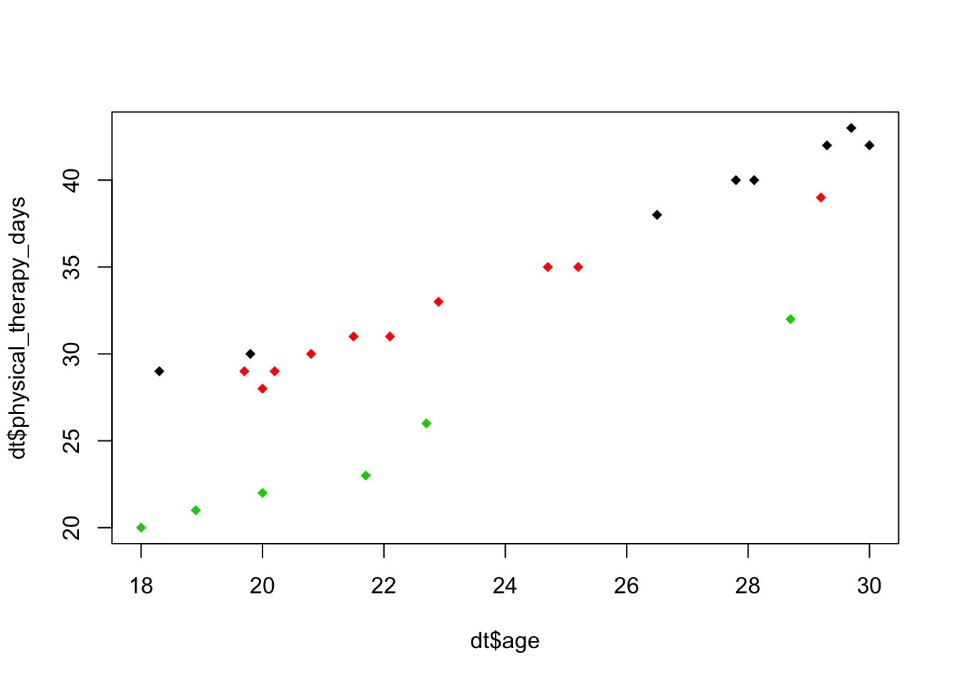
- Plot below also indicates no interaction effect
plot(dt$physical_therapy_days~dt$age, col=dt$fitness_status, pch=18)
Problem c
test for relationship between covariate and response variable
- The covariate is significantly correlated with the response variable.
cortest = cor.test(dt$physical_therapy_days,dt$age)
cortest
##
##  Pearson's product-moment correlation
##
## data:  dt$physical_therapy_days and dt$age
## t = 8.5376, df = 22, p-value = 1.972e-08
## alternative hypothesis: true correlation is not equal to 0
## 95 percent confidence interval:
##  0.7317657 0.9455402
## sample estimates:
##       cor
## 0.8764434
- correlation coefficient = 0.8764434, p-value = 1.972299e-08
cortest$estimate
##       cor
## 0.8764434
cortest$p.value
## [1] 1.972299e-08
Problem d
test for treatment effect
- There is a significant treatment effect on the physical therapy days
- F_star = 372.61, p-value = 2.257e-15
fit.treatment = aov(physical_therapy_days~age+fitness_status, dt)
variance_table = summary(fit.treatment)[[1]]
variance_table
##                Df Sum Sq Mean Sq F value    Pr(>F)
## age             1 835.75  835.75 2710.95 < 2.2e-16 ***
## fitness_status  2 246.08  123.04  399.11 < 2.2e-16 ***
## Residuals      20   6.17    0.31
## ---
## Signif. codes:  0 '***' 0.001 '**' 0.01 '*' 0.05 '.' 0.1 ' ' 1
variance_table[2,,drop=F]
##                Df Sum Sq Mean Sq F value    Pr(>F)
## fitness_status  2 246.08  123.04  399.11 < 2.2e-16 ***
## ---
## Signif. codes:  0 '***' 0.001 '**' 0.01 '*' 0.05 '.' 0.1 ' ' 1
Problem e
pairwise comparisons between treatment levels
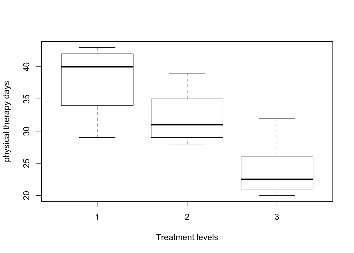
- All pairwise comparisons show significant difference.
fit.tukey = aov(physical_therapy_days~fitness_status, dt)
TukeyHSD(fit.tukey, conf.level = 0.95)
##   Tukey multiple comparisons of means
##     95% family-wise confidence level
##
## Fit: aov(formula = physical_therapy_days ~ fitness_status, data = dt)
##
## $fitness_status
##     diff       lwr        upr     p adj
## 2-1   -6 -11.32141 -0.6785856 0.0253639
## 3-1  -14 -20.05870 -7.9413032 0.0000254
## 3-2   -8 -13.79322 -2.2067778 0.0060547
boxplot(physical_therapy_days ~ fitness_status, dt, xlab="Treatment levels",
        ylab = "physical therapy days")
Copyright © 2017 Ming Chen & Wenqiang Feng. All rights reserved.