Homework #7

required library

library(car)

Load data

data65 <- read.table("./data/CH06PR05.txt", col.names = c("Y", "X1","X2"))

Problem 10.5(a)

• Added variable plots

lm.fit = lm(Y~., data=data65)
avPlots(lm.fit)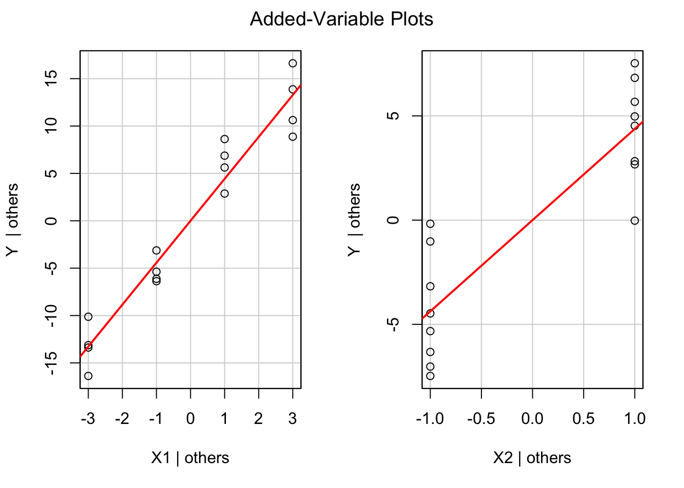

Problem 10.5(b)

• Explanation: The plots show a linear band with nonzero slope. Those plots indicate that a linear term in \(X_1\) may be helpful addition to the regression model already containing \(X_2\). It can be shown that the slope of the least squares line though the origin fitted to the plotted residual is the slope of the the plot in the figure. the regression coefficient of \(X_1\) if this variable were added to the regression model already containing \(X_2\). (book page.385)