Homework #9

required library

library(plyr)
library(lmtest)

Load data

dt <- read.table("./data/CH19PR16.txt", 
                      col.names =  c("time", "technician", "make", "disk_drive"))
dt[,2] = as.factor(dt[,2])
dt[,3] = as.factor(dt[,3])
dt[,4] = as.factor(dt[,4])

problem 19.16 a

fitted_values = ddply(dt, .(technician, make), summarize, 
      mean=mean(time))
fitted_values

##   technician make mean
## 1          1    1 59.8
## 2          1    2 47.8
## 3          1    3 58.4
## 4          2    1 48.4
## 5          2    2 61.2
## 6          2    3 56.2
## 7          3    1 60.2
## 8          3    2 60.8
## 9          3    3 49.6

problem 19.16 b

anova2way = aov(time~technician+make+technician:make, data=dt)
technician = rep(c("technician 1", "technician 2", "technician 3"), each=15)
make = rep(rep(c("make 1", "make 2", "make 3"), each=5), 3)
res=data.frame(technician, make, residuals=anova2way$residuals)
res

##      technician   make residuals
## 1  technician 1 make 1       2.2
## 2  technician 1 make 1     -11.8
## 3  technician 1 make 1       3.2
## 4  technician 1 make 1      -2.8
## 5  technician 1 make 1       9.2
## 6  technician 1 make 2       9.2
## 7  technician 1 make 2      -2.8
## 8  technician 1 make 2      -8.8
## 9  technician 1 make 2       6.2
## 10 technician 1 make 2      -3.8
## 11 technician 1 make 3       0.6
## 12 technician 1 make 3      -5.4
## 13 technician 1 make 3       8.6
## 14 technician 1 make 3       7.6
## 15 technician 1 make 3     -11.4
## 16 technician 2 make 1       2.6
## 17 technician 2 make 1       8.6
## 18 technician 2 make 1      -3.4
## 19 technician 2 make 1       1.6
## 20 technician 2 make 1      -9.4
## 21 technician 2 make 2      -0.2
## 22 technician 2 make 2      -3.2
## 23 technician 2 make 2       8.8
## 24 technician 2 make 2       4.8
## 25 technician 2 make 2     -10.2
## 26 technician 2 make 3      -1.2
## 27 technician 2 make 3       1.8
## 28 technician 2 make 3      -6.2
## 29 technician 2 make 3      12.8
## 30 technician 2 make 3      -7.2
## 31 technician 3 make 1      -1.2
## 32 technician 3 make 1       4.8
## 33 technician 3 make 1      -5.2
## 34 technician 3 make 1      -8.2
## 35 technician 3 make 1       9.8
## 36 technician 3 make 2      -2.8
## 37 technician 3 make 2       2.2
## 38 technician 3 make 2       9.2
## 39 technician 3 make 2      -7.8
## 40 technician 3 make 2      -0.8
## 41 technician 3 make 3      -2.6
## 42 technician 3 make 3       6.4
## 43 technician 3 make 3       1.4
## 44 technician 3 make 3      -5.6
## 45 technician 3 make 3       0.4

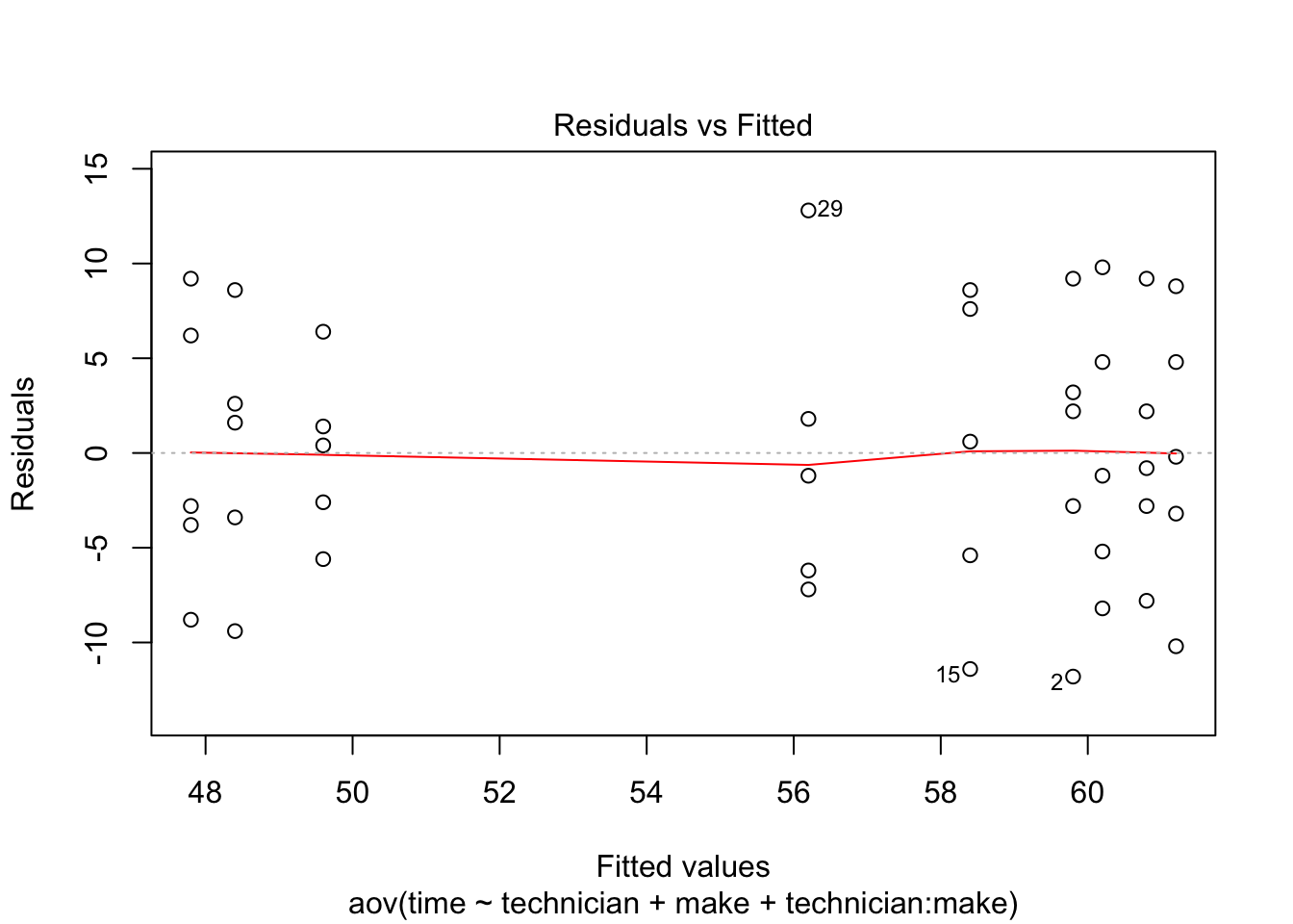
problem 19.16 c

Departures that can be studies * Nonconstancy of error variance * Nonindependency of error items * Outliers * Omission of important explanatory variables * Nonnormality of error terms

## plot residuals vs fitted value 
plot(anova2way, which=1)

problem 19.16 d

• Yes. the normality assumption appear to be reasonable here.
• Normal probability plot

plot(anova2way, which=2)

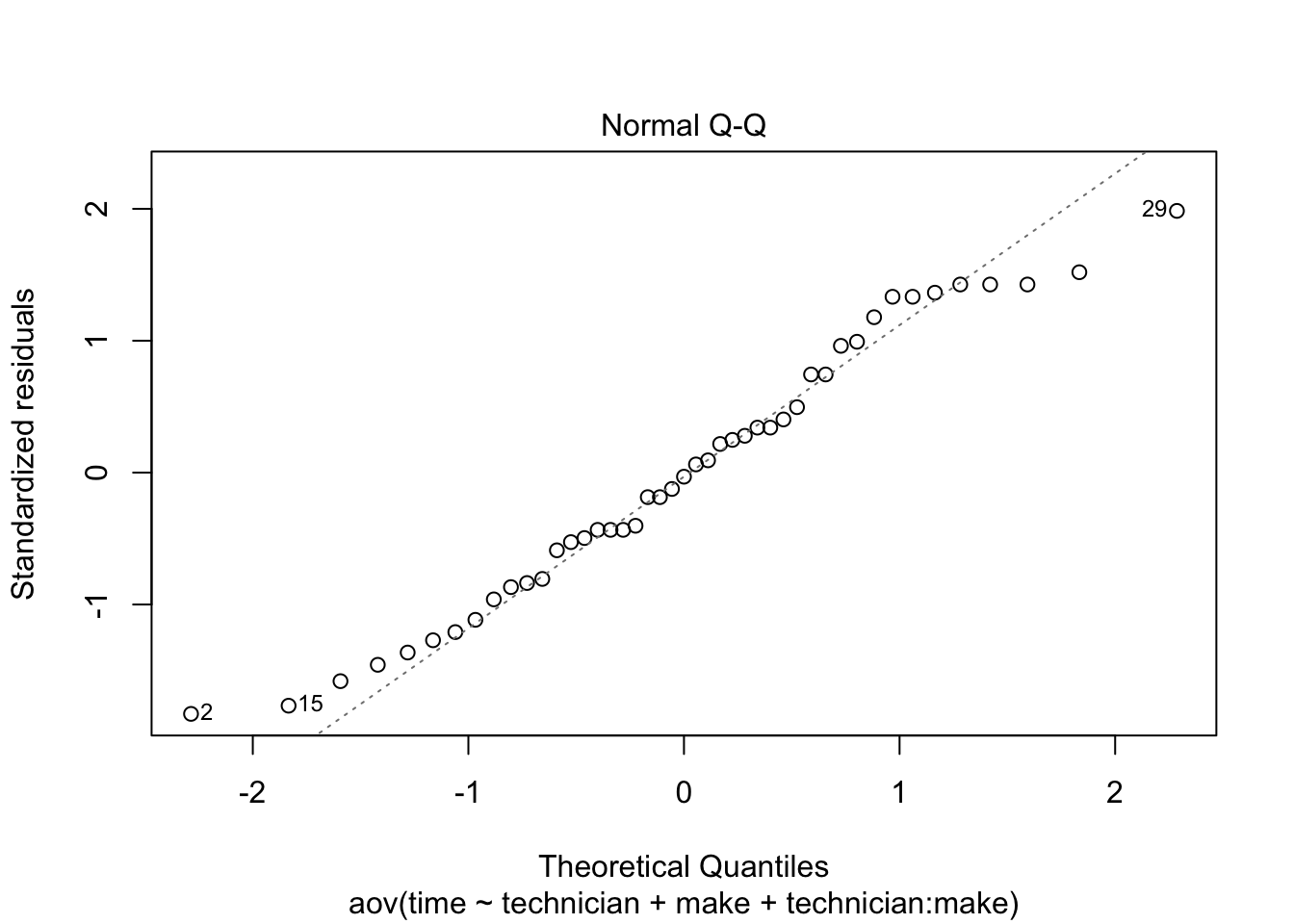
• Correlation coefficient = 0.9889246

lm.fit = lm(time~technician+make+technician:make, data=dt)
StdErr = summary(lm.fit)$sigma
n = length(res$residuals)
ExpVals = sapply(1:n, function(k) StdErr*qnorm((k-.375)/(n+.25)) )
r = cor(ExpVals, sort(res$residuals))
r

## [1] 0.9889246

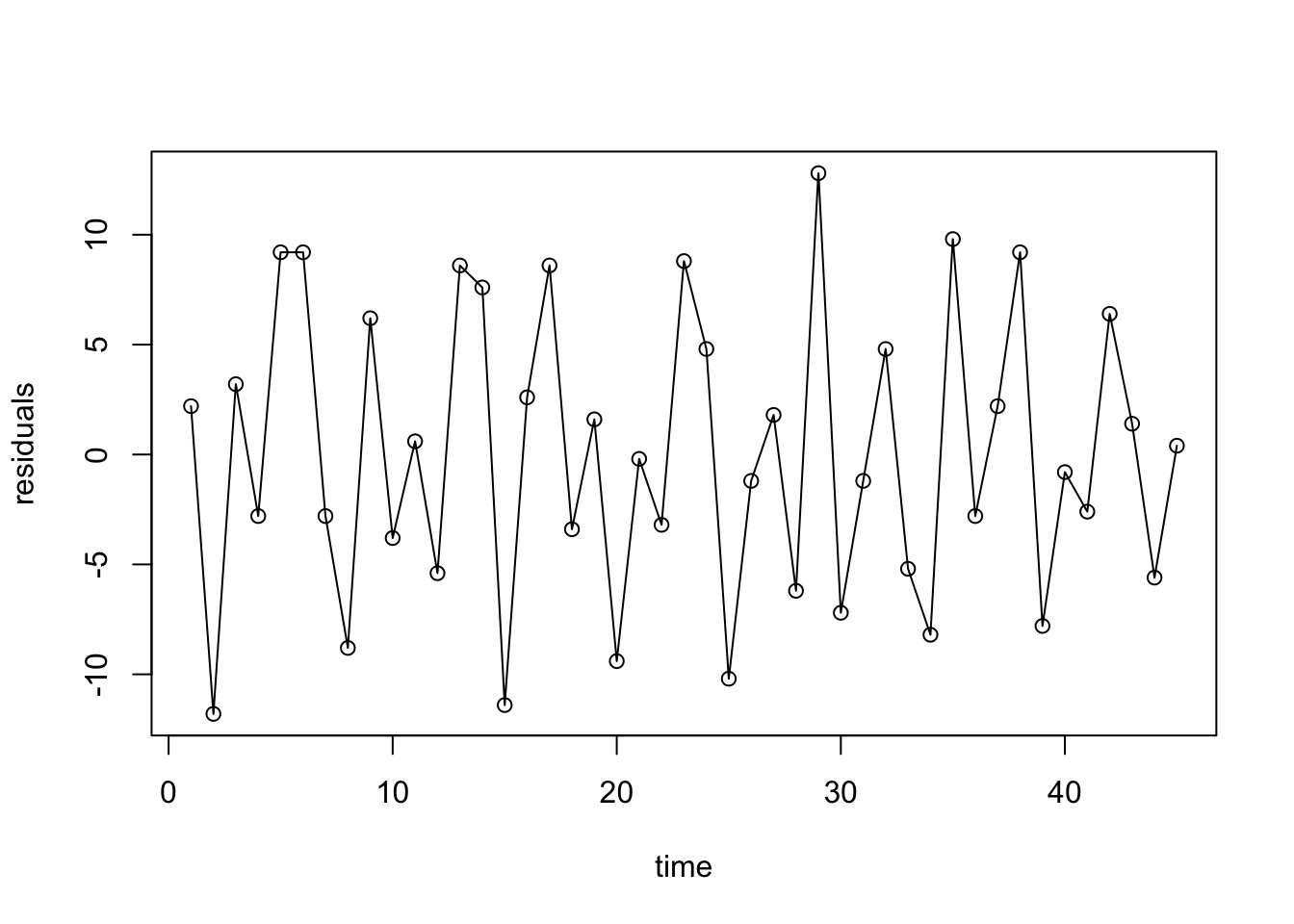
problem 19.16 e

• Residual sequence plots the residual sequence plot

plot(res$residuals, type="o", xlab="time", ylab="residuals")

par(mfrow=c(2,2))
plot(res$residuals[1:15], type="o", xlab="time order", ylab="residuals", main="Technician 1")
abline(h=0, col="gray")
plot(res$residuals[16:30], type="o", xlab="time order", ylab="residuals", main="Technician 2")
abline(h=0, col="gray")
plot(res$residuals[31:45], type="o", xlab="time order", ylab="residuals", main="Technician 3")
abline(h=0, col="gray")

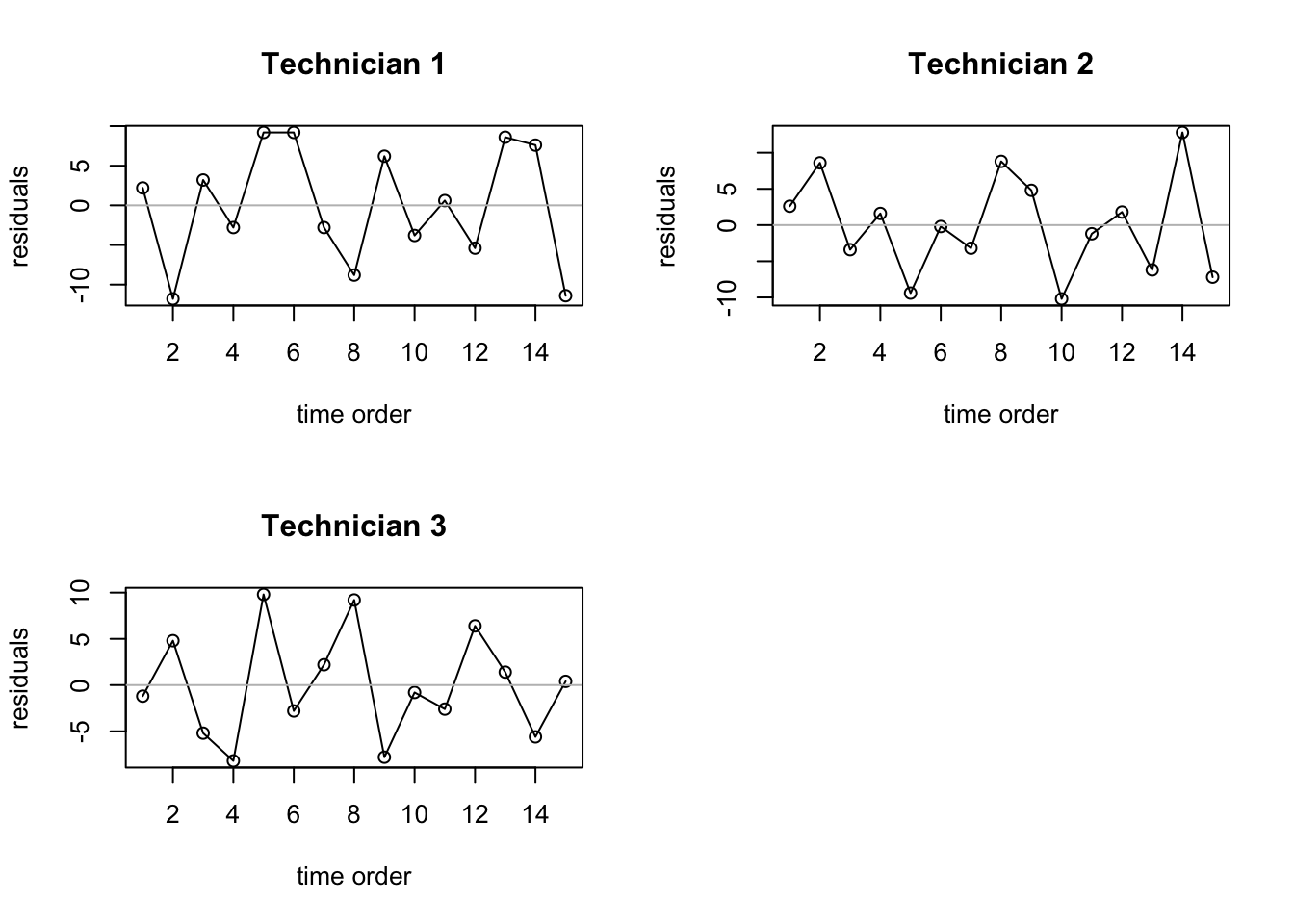
• All three plots show a random pattern. The residuals are not serially correlated.

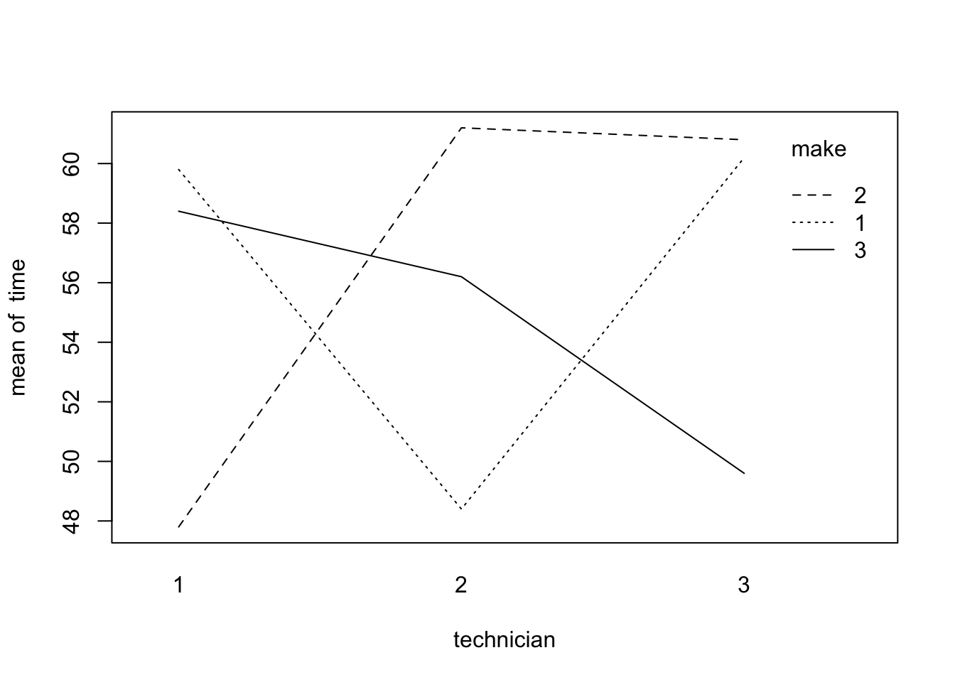
problem 19.17 a

Yes. Significant factor effect exists. The lines are not parallel to each other. There is a strong interaction effect between technician and make.

technician = dt$technician
make = dt$make
time = dt$time
interaction.plot(technician, make, time)

problem 19.17 b

Yes. the interaction term accounts for most of the total variability.

summary(anova2way)

##                 Df Sum Sq Mean Sq F value   Pr(>F)    
## technician       2   24.6   12.29   0.236 0.790779    
## make             2   28.3   14.16   0.272 0.763283    
## technician:make  4 1215.3  303.82   5.841 0.000994 ***
## Residuals       36 1872.4   52.01                     
## ---
## Signif. codes:  0 '***' 0.001 '**' 0.01 '*' 0.05 '.' 0.1 ' ' 1

problem 19.17 c

• alternatives
• H0: coefficients of all interaction terms equal zero

• Ha: not all coefficients of all interaction terms equal zero

• F_star = 303.82/52.01 = 5.841569

• for alpha=0.01, F(0.99; 4, 36) = 3.890308

qf(0.99, 4, 36)

## [1] 3.890308

• decision
• Conclude H0 if F_star > F(0.99; 4, 36)
• Conclude Ha if F_star < F(0.99; 4, 36)
• since F_star = 5.841569 > F(0.99; 4, 36) = 3.890308, conclude Ha.
• P value = 0.000994

summary(anova2way)[[1]]$Pr[3]

## [1] 0.0009941068

problem 19.17 d

qf(.99, 2, 36)

## [1] 5.247894

summary(anova2way)[[1]]$Pr[1]

## [1] 0.7907788

qf(.99, 2, 36)

## [1] 5.247894

summary(anova2way)[[1]]$Pr[2]

## [1] 0.7632826

problem 19.17 e

• upper bound = 1-(1-0.01)(1-0.01)(1-0.01) = 0.029701

problem 19.17 f

• yes. the p value for interaction item is less than 0.05, which indicates that there is a significant interaction effect. While the main effects are not significant.

problem 19.33 a

µ11 = [51.02908, 68.57092]

• explanation: there is a 99% chance that the average number of minutes required by technician 1 to repair make 1 of disk drive will be located within [51.02908, 68.57092].

• MSE = 52.01111

summary(anova2way)[[1]][3][4,]

## [1] 52.01111

• n = 5
• s{Y11.} = MSE/n = 3.225213
• t(0.995; 36) = 2.719485

qt(.995, 36)

## [1] 2.719485

• Y11 = 59.8

fitted_values$mean[1]

## [1] 59.8

• µ11 = [Y11-t(0.995; 36)*s{Y11.}, Y11+t(0.995; 36)*s{Y11.}]
  • Y11-t(0.995; 36)*s{Y11.} = 59.8 - 2.719485*3.225213 = 51.02908
  • Y11+t(0.995; 36)*s{Y11.} = 59.8 + 2.719485*3.225213 = 68.57092

problem 19.33 b

• s{D_hat} = (2*MSE/n)^0.5 = (2*52.01/5)^.5 = 4.56114
• D_hat = µ22 - µ21 = 61.2 - 48.4 = 12.8

## µ22
fitted_values$mean[5]

## [1] 61.2

## µ21
fitted_values$mean[4]

## [1] 48.4

• t(0.995; 36) = 2.719485

qt(0.995, 36)

## [1] 2.719485

• 99% confidence interval = [D_hat - t(0.995; 36) * s{D_hat}, D_hat + t(0.995; 36) * s{D_hat}]
  • 99% confidence interval = [0.3960482, 25.20395]
• explanation: there is a 99% chance that the difference between the average number of minitues needed by technician 2 and technician 1 to repaire make 1 of disc drive will be located within [0.3960482, 25.20395]. And technician 2 will need more time to repair the same make of disc drive.

problem 19.33 c

• D1 = µ11 - µ12 = 12
• D2 = µ11 - µ13 = 1.4
• D3 = µ12 - µ13 = -10.6
• D4 = µ21 - µ22 = -12.8
• D5 = µ21 - µ23 = -7.8
• D6 = µ22 - µ23 = 5.0
• D7 = µ31 - µ32 = -0.6
• D8 = µ31 - µ33 = 10.6

• D9 = µ32 - µ33 = 11.2

• s{D} = 4.56114

• t(1-0.1/(2*6); 36) = 2.51104

d = c(12, 1.4, -10.6, -12.6, -7.8, 5, -0.6, 10.6, 11.2)
s = 4.56114
t = 2.51104
ci = data.frame(lower = d-s*t, upper = d+s*t)
rownames(ci) = paste("D", 1:9, sep='')
ci

##         lower     upper
## D1   0.546795 23.453205
## D2 -10.053205 12.853205
## D3 -22.053205  0.853205
## D4 -24.053205 -1.146795
## D5 -19.253205  3.653205
## D6  -6.453205 16.453205
## D7 -12.053205 10.853205
## D8  -0.853205 22.053205
## D9  -0.253205 22.653205