Homework#13

require package

library(plyr)

Load data

dt <- read.table("./data/CH27PR13.txt", 
                col.names =  c("response", "store", "display", "time_period"))
dt$store = as.factor(dt$store)
dt$display = as.factor(dt$display)
dt$time_period = as.factor(dt$time_period)

Problem 27.13 a

• obtain residuals

fit = aov(response~display * time_period + Error(store/(display)), dt)
residuals = proj(fit)[[4]][, "Residuals"]
residuals = data.frame(id=dt$display, res=residuals)
residuals = arrange(residuals, id)
residuals = matrix(residuals$res, 8, 4, byrow=T)
colnames(residuals) =  c("k=1", "k=2", "k=3", "k=4")
rownames(residuals) = paste("i", c(1:4, 1:4), sep="=")
residuals

##         k=1    k=2     k=3     k=4
## i=1   9.250 -8.750   1.250  -1.750
## i=2 -11.750 -2.750  15.250  -0.750
## i=3   7.750 -5.250   5.750  -8.250
## i=4  -5.250 16.750 -22.250  10.750
## i=1   3.625 -3.125 -13.875  13.375
## i=2  15.375  6.625   7.875 -29.875
## i=3  -8.375 -3.125  -3.875  15.375
## i=4 -10.625 -0.375   9.875   1.125

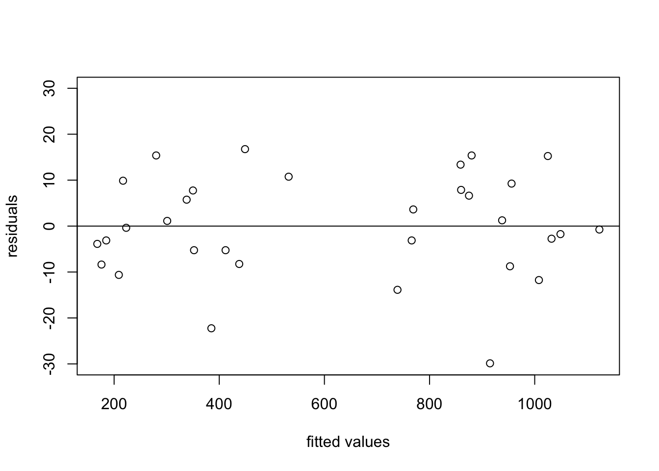
• residuals against the fitted values

plot(proj(fit)[[4]][, "Residuals"]~dt$response-proj(fit)[[4]][, "Residuals"], 
     xlab="fitted values", ylab="residuals", ylim=c(-30, 30))
abline(h=0)

• qqplot

qqnorm(qqplotData$y, ylim=c(-30, 30))
qqline(qqplotData$y)

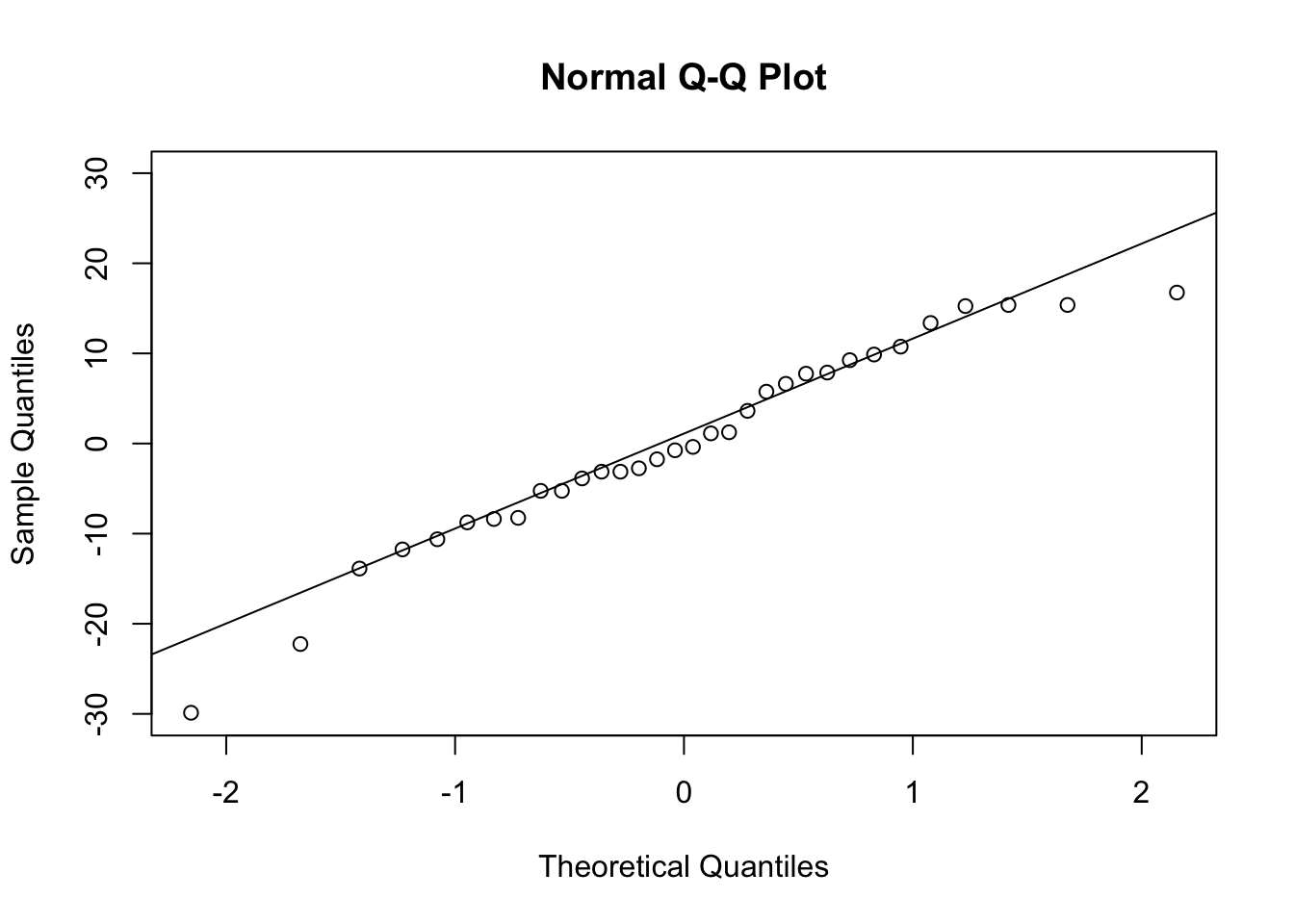
• Based on plots above, the model is appropriate to explain this data.

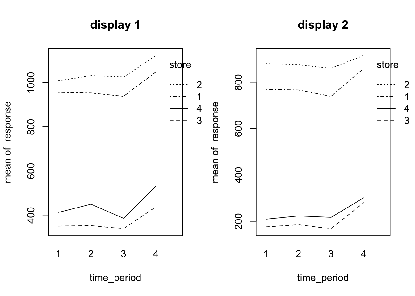
Problem 27.13 b

• Based on the plot, the model is appropriate here.

par(mfrow=c(1,2))
dat = subset(dt, display==1)
store = dat$store
time_period = dat$time_period
response = dat$response
interaction.plot(time_period, store, response, main="display 1")

dat = subset(dt, display==2)
store = dat$store
time_period = dat$time_period
response = dat$response
interaction.plot(time_period, store, response, main="display 2")

Problem 27.15 a

S_display = summary(fit)[[1]][[1]][1,] + summary(fit)[[2]][[1]][2,]
S_display[1,3] = S_display[1,2]/S_display[1,1]
S_display[1,4] = S_display[1,3]/summary(fit)[[3]][[1]][3,3]
S_display[1,5] = 0
variance_table = rbind(summary(fit)[[2]][[1]][1,], S_display,  summary(fit)[[3]][[1]])
rownames(variance_table) = c("display", "S(display)", "time period", 
                             "display:time period", "Error")
variance_table

##                     Df  Sum Sq Mean Sq   F value    Pr(>F)    
## display              1  266085  266085  325.8684 0.0003708 ***
## S(display)           6 3004019  500670 2355.9395 < 2.2e-16 ***
## time period          3   53322   17774   83.6363 9.216e-11 ***
## display:time period  3     691     230    1.0833 0.3813307    
## Error               18    3825     213                        
## ---
## Signif. codes:  0 '***' 0.001 '**' 0.01 '*' 0.05 '.' 0.1 ' ' 1

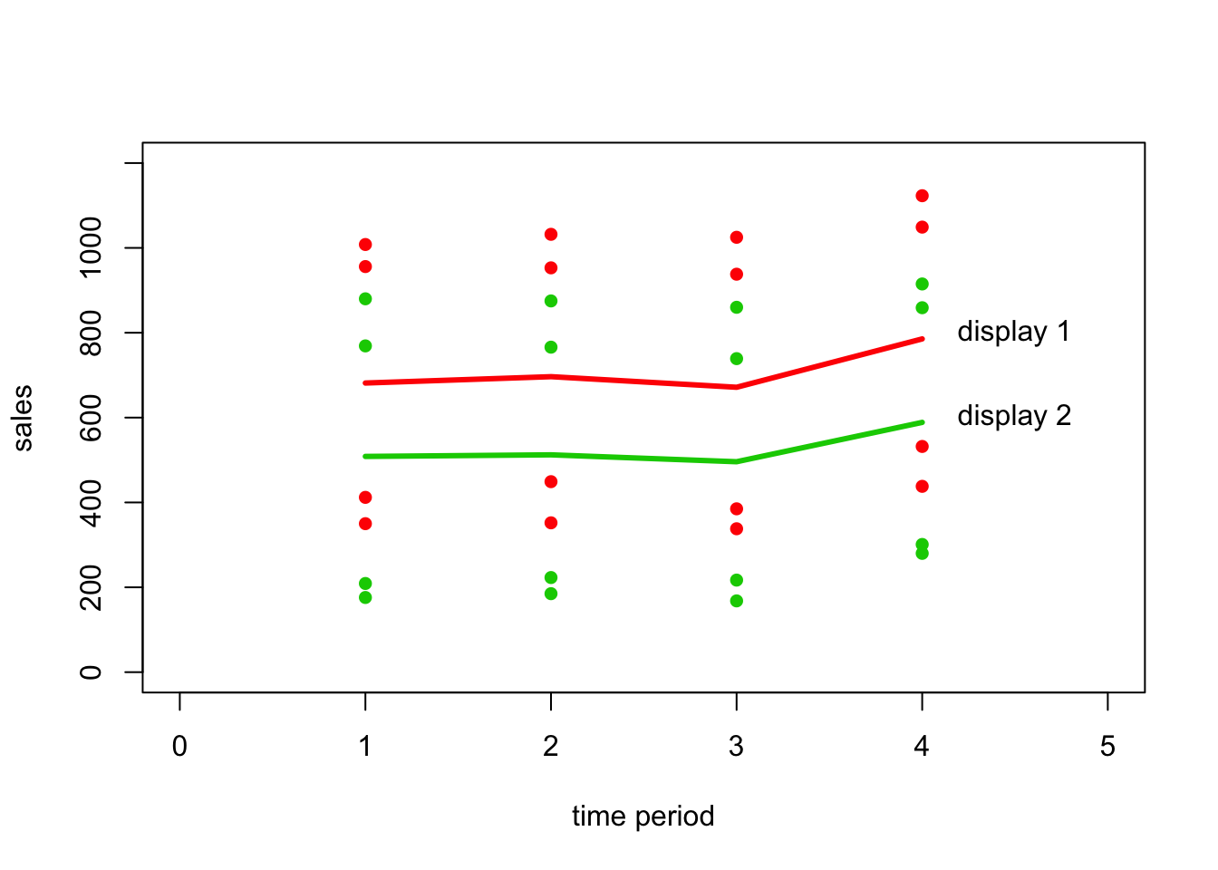
Problem 27.15 b

• No interaction effects
• Main effects exist

meanTime = ddply(dt, .(time_period, display), summarise, mean=mean(response))
dt <- read.table("./data/CH27PR13.txt", 
                col.names =  c("response", "store", "display", "time_period"))
plot(subset(dt, time_period==1&display==1)$time_period, subset(dt, time_period==1&display==1)$response, 
     xlim=c(0,5), ylim=c(0, 1200), xlab="time period", ylab = "sales", pch=16, col=2)
points(subset(dt, time_period==2&display==1)$time_period, subset(dt, time_period==2&display==1)$response, 
       xlim=c(0,5), ylim=c(0, 1200), xlab="time period", ylab = "sales", pch=16, col=2)
points(subset(dt, time_period==3&display==1)$time_period, subset(dt, time_period==3&display==1)$response, 
       xlim=c(0,5), ylim=c(0, 1200), xlab="time period", ylab = "sales", pch=16, col=2)
points(subset(dt, time_period==4&display==1)$time_period, subset(dt, time_period==4&display==1)$response, 
       xlim=c(0,5), ylim=c(0, 1200), xlab="time period", ylab = "sales", pch=16, col=2)

mean1 = subset(meanTime, display==1)
points(mean1$mean~mean1$time_period, type='l', col=2, lwd=3)
points(subset(dt, time_period==1&display==2)$time_period, subset(dt, time_period==1&display==2)$response, 
       xlim=c(0,5), ylim=c(0, 1200), xlab="time period", ylab = "sales", pch=16, col=3)
points(subset(dt, time_period==2&display==2)$time_period, subset(dt, time_period==2&display==2)$response, 
       xlim=c(0,5), ylim=c(0, 1200), xlab="time period", ylab = "sales", pch=16, col=3)
points(subset(dt, time_period==3&display==2)$time_period, subset(dt, time_period==3&display==2)$response, 
       xlim=c(0,5), ylim=c(0, 1200), xlab="time period", ylab = "sales", pch=16, col=3)
points(subset(dt, time_period==4&display==2)$time_period, subset(dt, time_period==4&display==2)$response, 
       xlim=c(0,5), ylim=c(0, 1200), xlab="time period", ylab = "sales", pch=16, col=3)

mean2 = subset(meanTime, display==2)
points(mean2$mean~mean2$time_period, type='l', col=3, lwd=3)
text(4.5, 800, 'display 1')
text(4.5, 600, 'display 2')

Problem 27.13 c

• alternatives
  • H0: all (alpha*beta)jk equal zero
  • Ha: not all (alpha*beta)jk equal zero
• decision rules: if F_star <= F(.975; 3, 18), conclude H0; otherwise, conclude Ha.
• conclusion: F_star = 1.083 < F(.975; 3, 18) = 3.953863, conclude H0.
• pvalue = 0.381

summary(fit)[[3]][1]

##                     Df Sum Sq Mean Sq F value   Pr(>F)    
## time_period          3  53322   17774  83.636 9.22e-11 ***
## display:time_period  3    691     230   1.083    0.381    
## Residuals           18   3825     213                     
## ---
## Signif. codes:  0 '***' 0.001 '**' 0.01 '*' 0.05 '.' 0.1 ' ' 1

Problem 27.13 d

• alternatives
  • H0: all (alpha)j equal zero
  • Ha: not all (alpha)j equal zero
• decision rules: if F_star <= F(.975; 1, 6), conclude H0; otherwise, conclude Ha.
• conclusion: F_star = 1.083 < F(.95; 1, 6) = 8.813101, conclude H0.
• pvalue = 0.3813

summary(fit)[[3]][[1]][2,]

##                     Df Sum Sq Mean Sq F value Pr(>F)
## display:time_period  3 690.62  230.21  1.0833 0.3813

• alternatives
  • H0: all (beta)j equal zero
  • Ha: not all (beta)j equal zero
• decision rules: if F_star <= F(.975; 1, 6), conclude H0; otherwise, conclude Ha.
• conclusion: F_star = 83.636 > F(.95; 1, 6) = 8.813101, conclude Ha.
• pvalue = 9.22e-11

summary(fit)[[3]][[1]][1,4, drop=FALSE]

##                     F value
## time_period          83.636

Problem 27.15 e

• L1 = 182.375
• L2 = -9.375
• L3 = 20.625
• L4 = -103.375
• s = 4
• a = 2
• b = 4
• s{Li} = 2MSB.S(A)/as = ((2*213)/(2*4))^.5 = 7.29726
• s{L1} = 2MSS(A)/bs = ((2*213)/(2*4))^.5 = 250.1674
• Bi = t(.9875; 18) = 2.445006
• B1 = t(.9875, 6) = 2.968687
• Confidence intervals
  • L1 = [L1-s{L1}B1, L1+s{L1}B1] = [-560.2937, 925.0437], no significant difference
  • L2 = [L2-s{Li}Bi, L2+s{Li}Bi] = [-27.21684, 8.466844], no significant difference
  • L3 = [L3-s{Li}Bi, L3+s{Li}Bi] = [2.783156, 38.46684], significant difference
  • L4 = [L4-s{Li}Bi, L4+s{Li}Bi] = [-121.2168, -85.53316], significant difference

L = ddply(dt, .(display), summarise, mu = mean(response))
L1 = L$mu[1] - L$mu[2]
L1

## [1] 182.375

L = ddply(dt, .(time_period), summarise, mu = mean(response))
L2 = L$mu[1] - L$mu[2]
L2

## [1] -9.375

L3 = L$mu[2] - L$mu[3]
L3

## [1] 20.625

L4 = L$mu[3] - L$mu[4]
L4

## [1] -103.375