Homework #3
Ming Chen & Wenqiang Feng
2/2/2017
1. Chapter 6 Problems 5abcd
Load data
data65 <- read.table("./data/CH06PR05.txt", col.names = c("y", "x1","x2"))- Problem 6.5 (a)
Scatter plot matrix and correlation matrix
- Scatter plot matrix
library(ggplot2)
pairs(data65, col="gray20")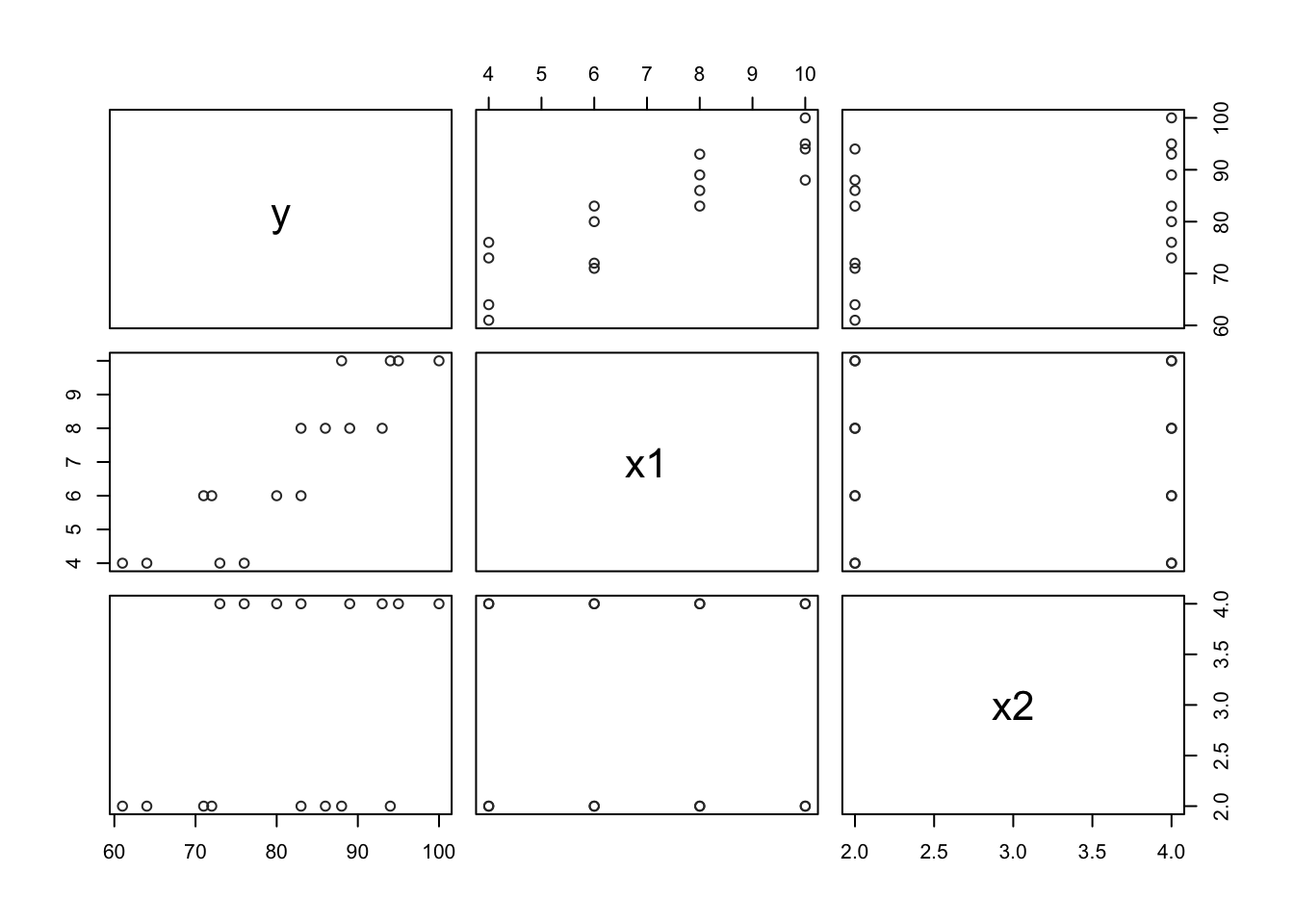
- Correlation matrix
cor(data65)## y x1 x2
## y 1.0000000 0.8923929 0.3945807
## x1 0.8923929 1.0000000 0.0000000
## x2 0.3945807 0.0000000 1.0000000Information from these diagnostic aids: From the correlation matrix, we can conclude that Y (branding linking) is positively correlated to \(X_1\) (mosture content) and \(X_2\) (sweetness). Moreover, The correlation is stronger between Y and \(X_1\) (0.89) than between Y and \(X_2\) (0.39) and no correlation between \(X_1\) and \(X_2\).
Problem 6.5 (b)
Fit regression model
lm.fit = lm(y~x1+x2, data=data65)
summary(lm.fit)
##
## Call:
## lm(formula = y ~ x1 + x2, data = data65)
##
## Residuals:
## Min 1Q Median 3Q Max
## -4.400 -1.762 0.025 1.587 4.200
##
## Coefficients:
## Estimate Std. Error t value Pr(>|t|)
## (Intercept) 37.6500 2.9961 12.566 1.20e-08 ***
## x1 4.4250 0.3011 14.695 1.78e-09 ***
## x2 4.3750 0.6733 6.498 2.01e-05 ***
## ---
## Signif. codes: 0 '***' 0.001 '**' 0.01 '*' 0.05 '.' 0.1 ' ' 1
##
## Residual standard error: 2.693 on 13 degrees of freedom
## Multiple R-squared: 0.9521, Adjusted R-squared: 0.9447
## F-statistic: 129.1 on 2 and 13 DF, p-value: 2.658e-09- Coefficients
beta=coef(lm.fit)
names(beta) = c("b0", "b1", "b2")
beta
## b0 b1 b2
## 37.650 4.425 4.375- Regression function
#Y_hat = beta[1] + beta[2]*X1 + beta[3]*X2\[ \hat{Y} = 37.65 + 4.425*X_1 + 4.375*X_2 \]
- Interpretation of b1
The coefficient \(b_1\) represents that when \(X_1\) (mosture content) increasing or descreasing by 1 unit, the Y (branding linking) will increase or descrease by 4.425 unit (under the assumption that the other variables are fixed).
Problem 6.5 (c)
Residuals and boxplot of residuals
residuals = lm.fit$residuals
residuals
## 1 2 3 4 5 6 7 8 9 10 11 12
## -0.10 0.15 -3.10 3.15 -0.95 -1.70 -1.95 1.30 1.20 -1.55 4.20 2.45
## 13 14 15 16
## -2.65 -4.40 3.35 0.60boxplot(residuals)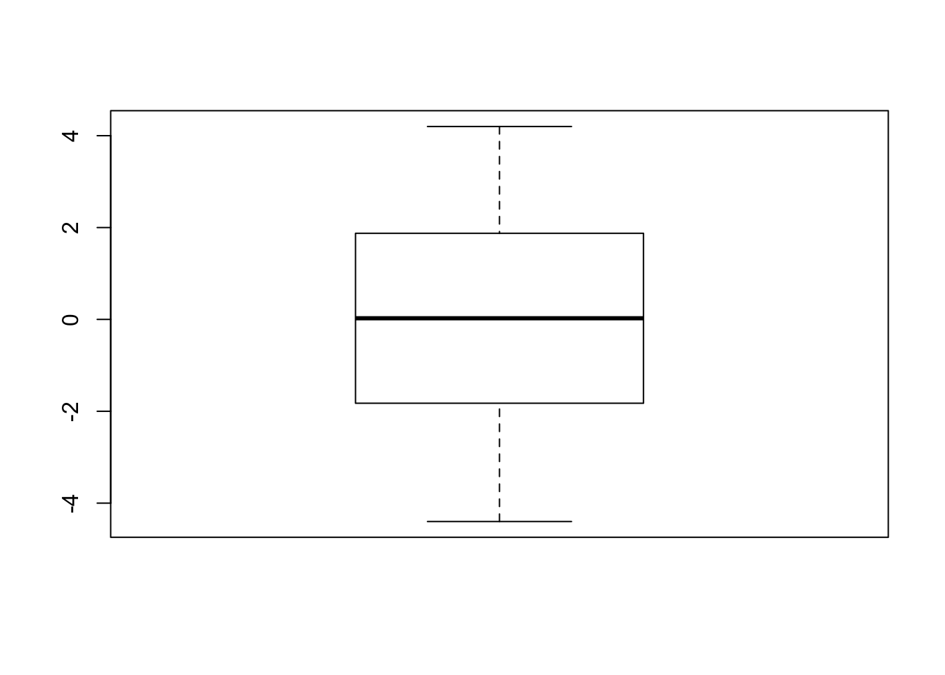
Y_hat = predict(lm.fit)
Y_hat
## 1 2 3 4 5 6 7 8 9 10 11 12
## 64.10 72.85 64.10 72.85 72.95 81.70 72.95 81.70 81.80 90.55 81.80 90.55
## 13 14 15 16
## 90.65 99.40 90.65 99.40- Information provided by box plot
The above boxplot indicates that the number of positive and negative residuals are about to be equal and no outliers in this data. Moreover, the residuals are evenly distributed and centered around 0. Hence, we can conclude that the regression model fits the data well.
problem 6.5 (d)
- Residual plots against \(\hat{Y}, X_1, X_2\) and \(X_1X_2\) on separate graphs
layout(matrix(c(1,2,1,2,3,4,3,4), 4,2, byrow=TRUE))
X1 = data65$x1
X2 = data65$x2
X1X2 = X1*X2
plot(residuals~Y_hat, ylim=c(-8,8), pch=20)
abline(h=0, lty=3, col=2)
plot(residuals~X1, ylim=c(-8,8), pch=20)
abline(h=0, lty=3, col=2)
plot(residuals~X2, ylim=c(-8,8), pch=20)
abline(h=0, lty=3, col=2)
plot(residuals~X1X2, ylim=c(-8,8), pch=20)
abline(h=0, lty=3, col=2)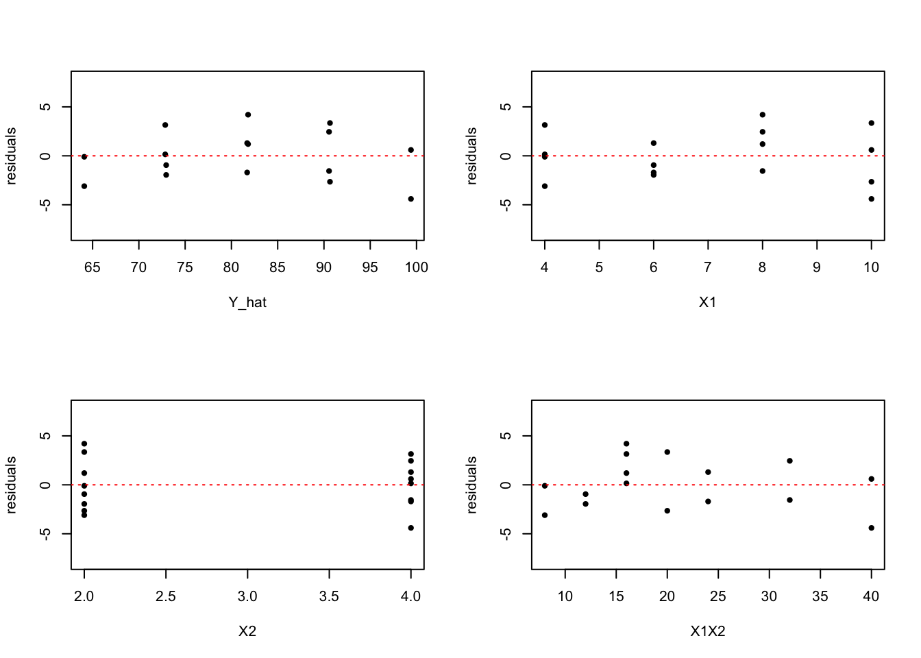
- Interpertation of residual plots
The upper left plot indicates that the variance of error terms does not vary with the level of Y hat. But there is a systematic pattern in the plot. The same pattern is found in the bottom right plot, which indicats that there is interaction effect.
2. Chapter 6 Problems 6
problem 6.6 (a)
F test for regression relation
- Hypothesis
- \(H_0\): \(\beta_1\) = \(\beta_2\) = 0, \(H_{\alpha}\): not all \(\beta_i\) = 0 (i=1,2)
- test statistic (\(\alpha =0.01, n=16, p=3\)): \[F^* = \frac{MSR}{MSE}.\]
- If \(F^* \leq F(1-\alpha; p-1, n-p) = F(0.99, 2, 13)\), conclude \(H_0\),
- If \(F^* > F(1-\alpha; p-1, n-p) = F(0.99, 2, 13)\) conclude \(H_a\).
- Calcuate of MSR and MSE \[\begin{eqnarray} SSE &=& e'e = (Y-Xb)'(Y-Xb) =Y'Y-b'X'Y'= Y'(I-H)Y\\ SSR &=& b'X'Y -\frac{1}{n}Y'JY = Y'\left[H-\frac{1}{n}J\right]Y \end{eqnarray}\]
mystats <- function (X,Y){
# reference : book page 225
XPrime <- t(X) #transposing X
YPrime <- t(Y) #transposing Y
n <- length(Y)  #here we assign our n
I <- matrix(0, nrow = n, ncol = n)  #we define an n by n
                          #matrix here that has an entries of 0.
I[row(I) == col(I)] <- 1  #here we assign a value 1 if the ith
                          #rows is equal to the jth columns.
J <- matrix(1, nrow = n, ncol = n)

#We are almost ready for computation, but before that we need
#to define first our H. To do that lets define the inverse
#first.

XXPrime <- XPrime%*%X       #here we define X’X
Inverse <- solve(XXPrime)   #here we have (X’X)^(-1)
H <- X%*%Inverse%*%XPrime

# SSR
SSRCen <- H - J/n  #here we define (H – J/n)
SSR <- YPrime%*%SSRCen%*%Y

# SSE
SSECen <- I - H  #here we define (I – H)
SSE <- YPrime%*%SSECen%*%Y

# MSR
MSR = SSR/(p-1)
# MSE
MSE = SSE/(n-p)
return(list(SSR=SSR,SSE=SSE,MSR=MSR, MSE=MSE))
}
p = 3
X <- as.matrix(cbind(1,data65[,2:3]))
Y <- as.matrix(data65[,1])
stats=mystats(X,Y)
stats$MSR## [,1]
## [1,] 936.35stats$MSE## [,1]
## [1,] 7.253846F_star = stats$MSR/stats$MSE
F_star## [,1]
## [1,] 129.0832- calculating \(F^* = \frac{MSR}{MSE} = \frac{936.35}{7.2538462}= {129.083245}\)
Remark: We can directly get the \(F^*\) value from summary of model fitting :
F_star = summary(lm.fit)$fstatistic[1]
F_star
## value
## 129.0832- calculating F(0.99; 5,8)
qf(0.99, 2,13)## [1] 6.700965- test results \(F^*\)= 129.083245 < F(0.99, 2, 13)= 6.7009645, Hence, we conclude \(H_{\alpha}\). That is to say the test results indicate that at least one of \(\beta_i\) (i=1,2) is not 0.
Problem 6.6 (b)
- P-value
p_value = 1 - pf(F_star,2,13)
p_value
## value
## 2.658261e-09Problem 6.6 (c)
- calculate s{b1}:s_b1 and s{b2}:s_b2
lm.fit = lm(y~., data=data65)
X = as.matrix(cbind(1, data65[,2:3]))
MSE = sum(lm.fit$residuals^2)/(nrow(data65)-3)
s_squared_b = MSE * solve(t(X)%*%X)
s_b1 = s_squared_b[2,2]^.5
s_b2 = s_squared_b[3,3]^.5- beta1 and beta2
beta1=coef(lm.fit)[2]
beta1
## x1
## 4.425beta2=coef(lm.fit)[3]
beta2## x2
## 4.375- Since \(\alpha =0.01\), then t_star=t(0.9975, 13)
t_star=qt(0.9975, 13)
t_star
## [1] 3.372468- Calculate 99% interval
beta1_lower = beta1-t_star*s_b1
beta1_upper = beta1+t_star*s_b1
beta1_interval=c(beta1_lower, "upper limit"=beta1_upper)
names(beta1_interval) = c("lower limit", "upper limit")- 99% CI for \(\beta_1\)
\[ 4.425 \pm 3.3724679 \cdot 0.3011197 \]
beta2_lower = beta2-t_star*s_b2
beta2_upper = beta2+t_star*s_b2
beta2_interval=c(beta2_lower, "upper limit"=beta2_upper)
names(beta2_interval) = c("lower limit", "upper limit")

beta1_interval
## lower limit upper limit
## 3.409483 5.440517beta2_interval## lower limit upper limit
## 2.104236 6.645764- 99% CI for \(\beta_2\)
\[4.375 \pm 3.3724679 \cdot 0.6733241 \]
- Interpretation:
- there is 99% confidence that the true \(\beta_1\) will be between 3.4094834 and 5.4405166
- there is 99% confidence that the true \(\beta_2\) will be between 2.104236 and 6.645764.
3. Chapter 6 Problems 7
Problem 6.7 (a)
- multiple determination \(R^2\) The model explains 95.2059% of the response variable variation.
R_squared = summary(lm.fit)$r.squared
R_adj_squared = summary(lm.fit)$adj.r.squared
R_squared
## [1] 0.952059R_adj_squared## [1] 0.9446834Problem 6.7 (b)
lm2.fit = lm(data65$y~Y_hat)
simple.dtm = c(summary(lm2.fit)$r.squared, summary(lm(data65$y~Y_hat))$adj.r.squared)
multiple.dtm = c(R_squared, R_adj_squared)
determination = cbind(simple_determination=simple.dtm, multiple_determination=multiple.dtm)
rownames(determination) = c("R squared", "adj R squared")
determination
## simple_determination multiple_determination
## R squared 0.9520590 0.9520590
## adj R squared 0.9486346 0.9446834- simple determination \(R^2\) between Y and \(\hat{Y}\) is 0.952059.
- Yes. The simple determination \(R^2\) equals the coefficient of multiple determination in part (a).
4. Chapter 6 Problems 8
Problem 6.8(a)
Y_interval_est_1 = predict(lm.fit, data.frame(x1=5, x2=4),
                           interval="confidence", level=0.99)
Y_interval_est_1
## fit lwr upr
## 1 77.275 73.88111 80.66889- The interval estimate of \(E[Y_h]\) is \(73.8811087 \leq E[Y_h] \leq 80.6688913\)
- Interpretation: there is 99% confidence that the true response value is between 73.8811087 and 80.6688913
Problem 6.8(b)
Y_interval_est_2 = predict(lm.fit, data.frame(x1=5, x2=4),
                           interval="prediction", level=0.99)
Y_interval_est_2
## fit lwr upr
## 1 77.275 68.48077 86.06923- The interval estimate of \(E[Y_{h(new)}]\) is \(68.4807696 \leq E[Y_{h(new)}] \leq 86.0692304\)
- Interpretation: there is 99% confidence that the true response value is between 68.4807696 and 86.0692304