require package
library(plyr)
library(asbio)
Load data
dt <- read.table("./data/CH27PR06.txt",
                col.names =  c("sales", "stores", "price"))
dt$stores = as.factor(dt$stores)
dt$price = as.factor(dt$price)
Problem 27.6 a
Residuals and normality test
- The residual is normally distributed
fit = aov(sales~stores+price, dt)
residuals = matrix(fit$residuals, nrow=8, byrow=T)
shapiro.test(residuals)
##
##  Shapiro-Wilk normality test
##
## data:  residuals
## W = 0.9874, p-value = 0.9861
Problem 27.6 b
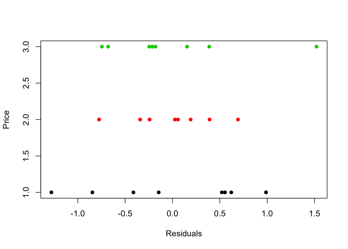
Aligned residual dot plots
- Yes. The plot supports the assumption of constancy of the error variance
plot(as.numeric(dt$price)~fit$residuals, xlab="Residuals", ylab="Price", col=dt$price, pch=16)
Problem 27.6 c
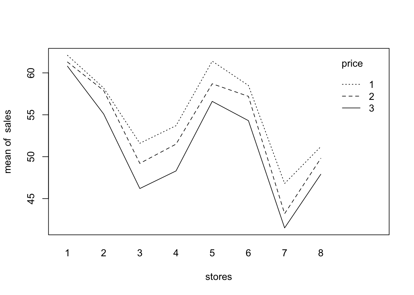
Interaction between subjects and treatments
- Yes. the assumption of no interaction between subjects and treatments is reasonable.
stores = dt$stores
sales = dt$sales
price = dt$price
interaction.plot(stores, price, sales)
Problem 27.7 a
Analysis of variance table
fit = aov(sales~stores+price, dt)
variance_table = round(summary(fit)[[1]], 3)
variance_table
##             Df Sum Sq Mean Sq F value    Pr(>F)
## stores       7 745.18 106.455 155.693 < 2.2e-16 ***
## price        2  67.48  33.740  49.346 < 2.2e-16 ***
## Residuals   14   9.57   0.684
## ---
## Signif. codes:  0 '***' 0.001 '**' 0.01 '*' 0.05 '.' 0.1 ' ' 1
Problem 27.7 b
Whether or not the mean sales of grapefruits differ
- alternatives
- H0: all Tj equal zero
- Ha: not all Tj equal zero
- decision rules: if F_star <= F(.95; 2, 14), conclude H0; otherwise, conclude Ha.
- conclusion: F_star = 49.346 > F(.95; 2, 14) = 3.738892, conclude Ha.
- pvalue < 2.2e-16
variance_table
##             Df Sum Sq Mean Sq F value    Pr(>F)
## stores       7 745.18 106.455 155.693 < 2.2e-16 ***
## price        2  67.48  33.740  49.346 < 2.2e-16 ***
## Residuals   14   9.57   0.684
## ---
## Signif. codes:  0 '***' 0.001 '**' 0.01 '*' 0.05 '.' 0.1 ' ' 1
variance_table[2,,drop=F]
##             Df Sum Sq Mean Sq F value    Pr(>F)
## price        2 67.481   33.74  49.346 < 2.2e-16 ***
## ---
## Signif. codes:  0 '***' 0.001 '**' 0.01 '*' 0.05 '.' 0.1 ' ' 1
Problem 27.7 c
Pairwise comparisons of the price level means
- Tukey procedure was applied for the pairwise comparisons.
- All differences are significant
- The mean of level 1 is the largest and the mean of level 3 is the smallest.
- the differnce between level 1 and level 3 is the largest.
- Below is the results:
TukeyHSD(fit, "price", ordered=T)
##   Tukey multiple comparisons of means
##     95% family-wise confidence level
##     factor levels have been ordered
##
## Fit: aov(formula = sales ~ stores + price, data = dt)
##
## $price
##       diff       lwr      upr     p adj
## 2-3 2.2625 1.1803961 3.344604 0.0002275
## 1-3 4.1000 3.0178961 5.182104 0.0000003
## 1-2 1.8375 0.7553961 2.919604 0.0015069
Copyright © 2017 Ming Chen & Wenqiang Feng. All rights reserved.