Homework #8

1. Chapter 16 Problems 12

required library

library(plyr)
library(gplots)
library(asbio)

Load data

data1612 <- read.table("./data/CH16PR12.txt")[,1:2]
colnames(data1612) = c("time_lapse", "agent")

Problem 16

problem 16.12 a

the factor level means appear to differ
the variability of the observations is approximately the same for all factor levels

boxplot(time_lapse~agent, data=data1612, xlab="agent", ylab="tiem lapse")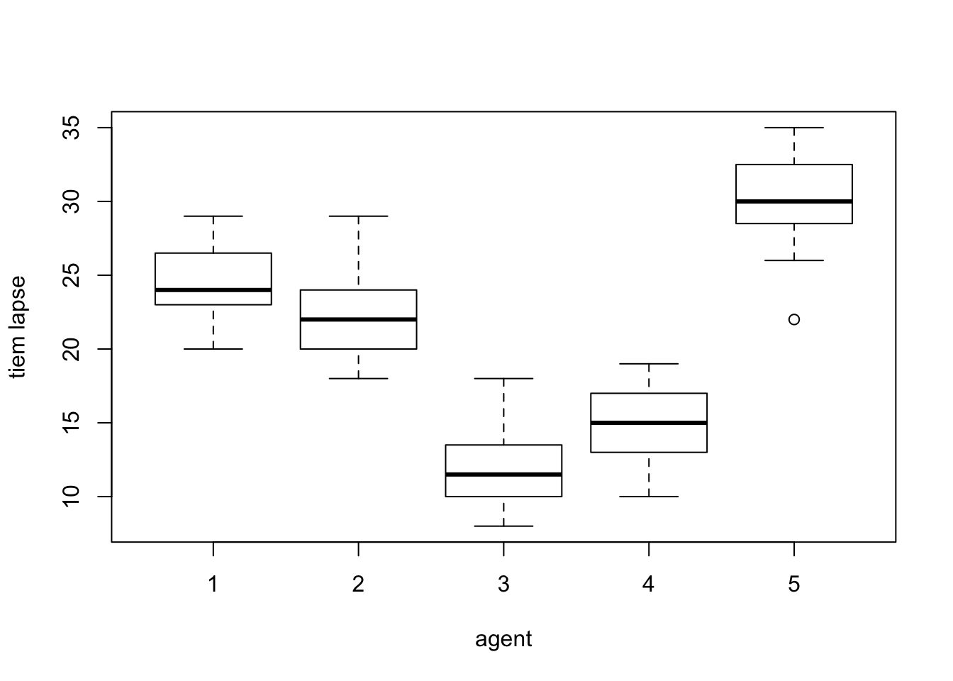

problem 16.12 b

data1612$agent = as.factor(data1612$agent)
aov.fit = aov(time_lapse~agent, data = data1612)
fitted_value = ddply(data1612, .(agent), summarize, mean=mean(time_lapse))
colnames(fitted_value) = c("agent", "fitted value") 
fitted_value

##   agent fitted value
## 1     1        24.55
## 2     2        22.55
## 3     3        11.75
## 4     4        14.80
## 5     5        30.10

problem 16.12 c

residuals

residuals = aov.fit$residuals
names(residuals) = rep(1:5, each=20)
matrix(residuals, nrow=20)

##        [,1]  [,2]  [,3] [,4] [,5]
##  [1,] -0.55 -4.55 -1.75  0.2  2.9
##  [2,] -0.55 -2.55 -0.75 -1.8 -8.1
##  [3,]  4.45 -2.55 -3.75  3.2 -2.1
##  [4,] -4.55  1.45  0.25  1.2  4.9
##  [5,] -3.55 -0.55  0.25 -2.8 -1.1
##  [6,]  0.45  6.45 -1.75  4.2 -2.1
##  [7,]  3.45  0.45  2.25 -4.8 -0.1
##  [8,]  2.45  1.45 -2.75  3.2  0.9
##  [9,] -1.55  5.45 -3.75 -3.8 -1.1
## [10,] -3.55 -3.55 -0.75  2.2 -2.1
## [11,] -0.55  1.45  4.25  0.2  2.9
## [12,]  1.45  2.45  0.25 -2.8 -0.1
## [13,] -1.55 -1.55  6.25 -1.8  1.9
## [14,] -0.55 -2.55  2.25 -1.8  2.9
## [15,]  3.45  1.45  1.25 -0.8 -1.1
## [16,] -1.55 -0.55 -0.75  2.2  4.9
## [17,] -1.55 -3.55  2.25  1.2  1.9
## [18,]  2.45  3.45 -2.75  2.2 -4.1
## [19,]  1.45 -0.55 -0.75 -0.8 -0.1
## [20,]  0.45 -1.55  0.25  1.2 -1.1

sum(residuals)

## [1] 3.802514e-15

Yes, the sum of residuals is $3.8025139\times 10^{-15}$ which is 0 at the machine error level.

problem 16.12 d

summary(aov.fit)

##             Df Sum Sq Mean Sq F value Pr(>F)    
## agent        4   4430  1107.5   147.2 <2e-16 ***
## Residuals   95    715     7.5                   
## ---
## Signif. codes:  0 '***' 0.001 '**' 0.01 '*' 0.05 '.' 0.1 ' ' 1

problem 16.12 e

Hypothesis:
$H_0$: all the $\mu_i, i= 1,\cdots,5$ are equal.
$H_\alpha$: not all $\mu_i, i= 1,\cdots,5$ are equal.
Decision rules: From the above ANOVA table , we get $F^*$ = 1107.5/7.5 = 147.6667; Now calculate F(0.90; 4, 95):

qf(0.90, 4, 95)

## [1] 2.004992

If $F^*$ is less or equal F(0.90; 4, 95)= 2.0049918, conclude $H_0$, otherwise $H_\alpha$. Based on this criteria, since $F^*$ = 147.6667 > 2.0049918, conclude $H_\alpha$.

problem 16.12 f

P value = 0

problem 16.12 g

Yes. There appears to be much variation in the mean time lapse among the five agents.
However, this variation does not necessarily indicate differences in the efficiency of operations of all five agents. It only means that at least one agent is significantly different from others.

1. Chapter 17 Problems 13

problem 17.13 a

The intervals of some agents are not overlapped with agents of any other agents, which indicates that there is a significant difference in time lapse among the five agents.

plotmeans(time_lapse~agent, data=data1612, xlab="agent", ylab="time lapse", p=0.9)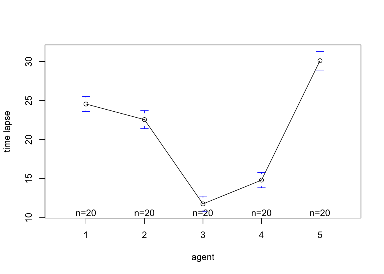

problem 17.13 b

given alpha = 0.1, so the confidence level = 0.90

tk.comparison = TukeyHSD(aov.fit, conf.level=0.90, ordered=T)
tk.comparison

##   Tukey multiple comparisons of means
##     90% family-wise confidence level
##     factor levels have been ordered
## 
## Fit: aov(formula = time_lapse ~ agent, data = data1612)
## 
## $agent
##      diff        lwr      upr     p adj
## 4-3  3.05  0.8845705  5.21543 0.0059245
## 2-3 10.80  8.6345705 12.96543 0.0000000
## 1-3 12.80 10.6345705 14.96543 0.0000000
## 5-3 18.35 16.1845705 20.51543 0.0000000
## 2-4  7.75  5.5845705  9.91543 0.0000000
## 1-4  9.75  7.5845705 11.91543 0.0000000
## 5-4 15.30 13.1345705 17.46543 0.0000000
## 1-2  2.00 -0.1654295  4.16543 0.1520498
## 5-2  7.55  5.3845705  9.71543 0.0000000
## 5-1  5.55  3.3845705  7.71543 0.0000001

based on the Tukey pairwised comparison, only the mean between group 1 and 2 do not differ

tk.comparison$agent[tk.comparison$agent[,4]>=0.05, , drop=FALSE]

##     diff        lwr     upr     p adj
## 1-2    2 -0.1654295 4.16543 0.1520498

groups
group 1: agent 1 and agent 2
group 2: agent 3
group 3: agent 4
group 4: agent 5

problem 17.13 f

No. Based on the table above, Bonferroni has narrower intervals than the tukey procedure.
Below is the plot of the entire result. Group pairs that intersect the dashed vertical line do not differ in time lapse mean. Here it is group pair (1, 2)

plot(tk.comparison)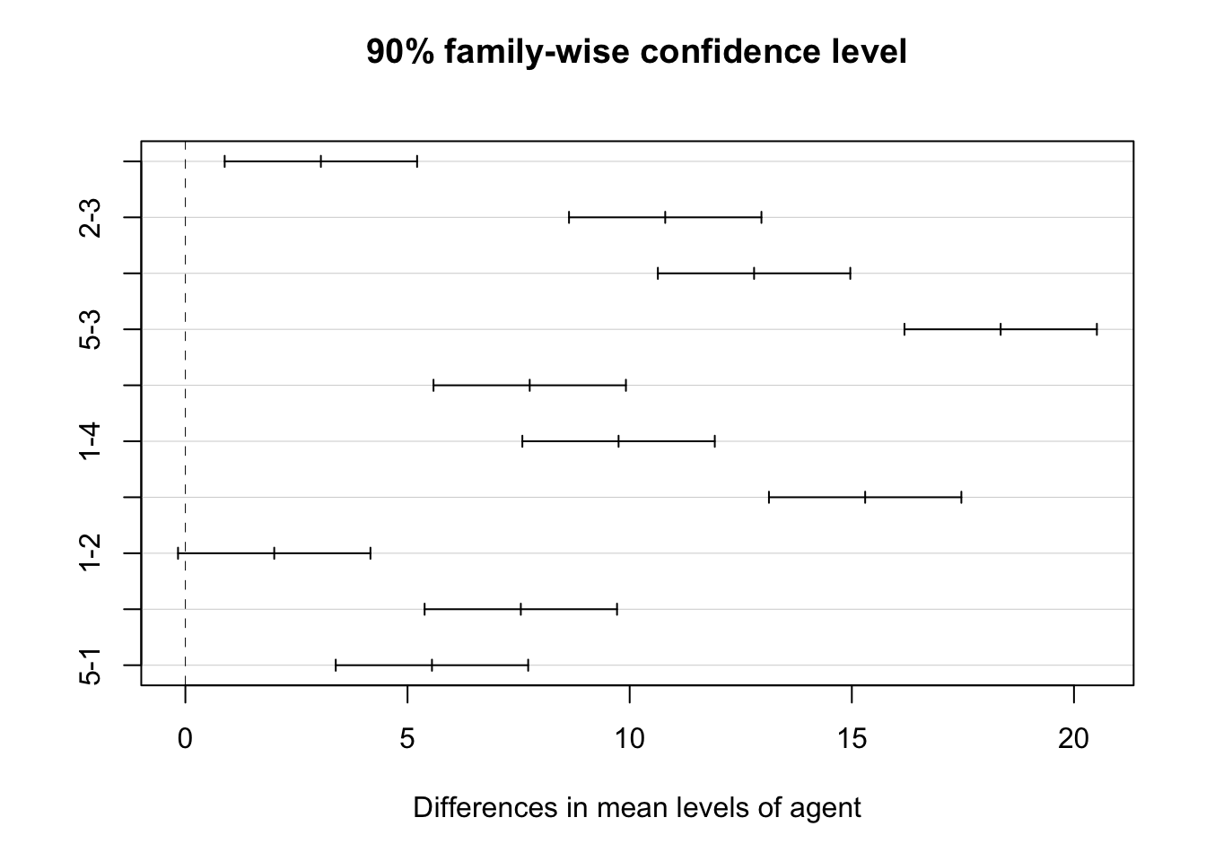

problem 17.13 c

MSE = 7.522632

MSE = summary(aov.fit)[[1]][3][2,1]
MSE

## [1] 7.522632

s{Y_bar1.} = $(MSE/20)^{0.5} = (7.522632/20)^{0.5}$ = 0.6132957
t(0.95, 95) = 1.661052

qt(0.95, 95)

## [1] 1.661052

c(24.550-(MSE/20)^(0.5)*qt(0.95, 95), 24.550+(MSE/20)^(0.5)*qt(0.95, 95))

## [1] 23.53128 25.56872

90% confidence interval = [23.53128 25.56872]
lower limit = Y1.mean - t(0.90, 95) * s{Y_bar1.} = 24.55 - 1.661052 * 0.6132957 = 23.53128
upper limit = Y1.mean + t(0.90, 95) * s{Y_bar1.} = 24.55 + 1.661052 * 0.6132957 = 25.56872

problem 17.13 d

D = mu2 - mu1 = 22.55 - 24.55 = -2
s{Y1.} = $(MSE/(1/20 + 1/20))^{0.5} $= 0.8673
t(0.95, 95) = 1.6610518
confidence interval: [D - t(0.90; 95) * s{Y1.}, [D - t(0.95; 95) * s{Y1.}] = [-3.441, -0.559]
explanation: the difference is significant. Time lapse for agent 2 is significantly less than that for agent 1.

problem 17.13 e

D1 = Y1 - Y3 = 12.8, 10.91794 < D1 < 14.607419
D2 = Y1 - Y5 = -5.55, -7.43206 < D2 < -3.66794
D3 = Y3 - Y5 = -18.35, -20.23206 < D3 < -16.46794
s{Di} = $(MSE*2/20)^{0.5}$ = 0.8673
B = t(1-0.1/2*3; 95) = t(0.9833; 95) = 2.158

\[ 12.8-2.158(0.8673) \leq D1 \leq 12.8+2.158(0.8673), 10.928 \leq D1 \leq 14.672 \] \[-5.55-2.158(0.8673) \leq D2 \leq -5.55+2.158(0.8673), -7.422 \leq D2 \leq -3.678\] \[-18.35-2.158(0.8673) \leq D3 \leq -18.35+2.158(0.8673), -20.222 \leq D3 \leq -16.478\]

Plot shows that all differences are significant. Same conclusions are obtained as in part(a).

D = c(12.8, -5.55, -18.35)
plot(cbind(D, 2), yaxt = "n", bty="l", ylab="", xlab="time lapse")
text(x=D, y=2.1, labels=1:3)
abline(h=2)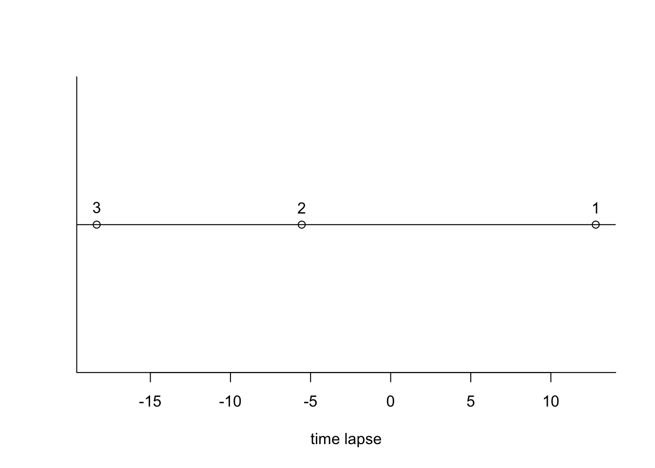

problem 17.13 f

No, since q(0.90, 5, 95) = 3.54, while T = 2.503.

1. Chapter 17 Problems 18

problem 17.18 a

mu1 = 24.55
mu2 = 22.55
mu3 = 11.75
mu4 = 14.80
L = (mu1+mu2)/2 - (mu3+mu4)/2 = 10.275
s{L} = $(MSE/n)^{0.5} = (7.522632/20)^{0.5}$ = 0.6132957
t(0.90, 95) = 1.290527
so, L confidence interval = [L - t(0.90, 95) * s{L}, L + t(0.90, 95) * s{L}] = [9.483526 11.066474]

mu1 = 24.55; mu2 = 22.55;mu3 = 11.75;mu4 = 14.80;n=20
L = (mu1+mu2)/2 - (mu3+mu4)/2
L

## [1] 10.275

sL = (MSE/n)^0.5
sL

## [1] 0.6132957

c(L - qt(0.90,95)*sL,L + qt(0.90, 95)*sL  )

## [1]  9.483526 11.066474

explanation: the time lapse is significantly different between agents who distribute merchandise only and agents who distribute cash-value coupons only.

mu = fitted_value[,2]
mu

## [1] 24.55 22.55 11.75 14.80 30.10

MSE

## [1] 7.522632

qt(0.90, 95)

## [1] 1.290527

problem 17.18 b

D1 = mu1 - mu2 = 24.55 - 22.55 = 2.00
D2 = mu3 - mu4 = 11.75 - 14.80 = -3.05
L1 = (mu1+mu2)/2 - mu5 = (24.55+22.55)/2 - 30.10 = -6.55
L2 = (mu3+mu4)/2 - mu5 = (11.75+14.80)/2 - 30.10 = -16.825
L3 = (mu1+mu2)/2 - (mu3+mu4)/2 = (24.55+22.55)/2 - (11.75+14.80)/2 = 10.275
s{D} = 0.8673
s{L1} = 0.7511
s{L3} = s{D} = 0.6133
F(0.90; 4, 95) = 2.004992
S = (4 * F(0.90; 4, 95))^0.5 = 2.831955
Using this formula: confidence interval = [L - S * s{L}, L + t(0.90, 95) * s{L}], we obtain the * following
confidence interval for each,
D1: [-0.4561543, 4.4561543]
D1: [-5.5061543, -0.5938457]
L1: [-8.6770812, -4.4229188]
L2: [-18.9520812, -14.6979188]
L3: [8.5381622, 12.0118378]

explanation: difference D1 is not significant. The others are significant.

mu = fitted_value[,2]
mu

## [1] 24.55 22.55 11.75 14.80 30.10

problem 17.18 c

L = 0.25mu1 + 0.20mu2 + 0.20mu3 + 0.20mu4 + 0.15mu5 = 20.4725
s{L} = 0.2777
t(0.90; 95) = 1.290527
L confidence interval: [L - t(0.90; 95) * s{L}, L + t(0.90; 95) * s{L}] = [20.114, 20.831]

L=sum(c(0.25, 0.2, .2, .2, .15)*fitted_value[,2])
L

## [1] 20.4725

qt(0.90, 95)

## [1] 1.290527

Homework #8

Wenqiang Feng

2/25/2017

1. Chapter 16 Problems 12

required library

Load data

Problem 16

problem 16.12 a

problem 16.12 b

problem 16.12 c

problem 16.12 d

problem 16.12 e

problem 16.12 f

problem 16.12 g

1. Chapter 17 Problems 13

problem 17.13 a

problem 17.13 b

problem 17.13 f

problem 17.13 c

problem 17.13 d

problem 17.13 e

problem 17.13 f

1. Chapter 17 Problems 18

problem 17.18 a

problem 17.18 b

problem 17.18 c